Profile Before You Optimize
By now we have built dozens of automata.
The natural temptation is to make them faster.
The wrong first question is:
Which optimization trick should I use?
The right first question is:
Where is the time actually going?
Performance work begins with measurement, and with the doctrine Part VI starts from:
Optimize the verified implementation, not the first implementation that happens to render something plausible.
Running this book’s own earlier code turned up undefined helpers, wrong signatures and a misaligned FFT, all inside chapters that produced plausible figures. Speed means nothing until equivalence is established.
Define the workload first
A benchmark is only meaningful if the workload is explicit.
For a cellular automaton, record at least:
grid size
number of channels
neighborhood radius
number of steps
data type
boundary rule
backend
A 64×64 Conway grid and a 1024×1024 multi-channel Lenia system are not the same performance problem.
Time one complete rollout
from time import perf_counter


def benchmark(step_fn, state, steps=200):
    x = state.copy()  # NumPy arrays; use .clone() for torch tensors

    start = perf_counter()
    for _ in range(steps):
        x = step_fn(x)
    elapsed = perf_counter() - start

    return {
        "seconds": elapsed,
        "steps_per_second": steps / elapsed,
        "seconds_per_step": elapsed / steps,
    }
(perf_counter is the right tool because it is the highest-resolution monotonic clock for short durations — not wall-clock time, which can jump.)
Run the benchmark several times.
The first run may include allocation, cache warm-up, kernel compilation or other one-time costs.
Measure scaling, not one number
Using Chapter 6’s life_step on random binary states:
def random_state(size, seed=0):
    rng = np.random.default_rng(seed)
    return rng.integers(0, 2, size=(size, size)).astype(np.uint8)


sizes = [64, 128, 256, 512]

for size in sizes:
    state = random_state(size)
    result = benchmark(life_step, state)
    print(size, result["steps_per_second"])
A scaling curve tells us much more than one headline number. Measured on one reference machine (life_step, 20 timed steps after warmup):
| Grid | Steps/s | ms/step | Work vs 64² |
|---|---|---|---|
| 64 | 10324 | 0.10 | 1× |
| 128 | 6461 | 0.15 | 4× cells, 1.6× slower |
| 256 | 2620 | 0.38 | 16× cells, 3.9× slower |
| 512 | 534 | 1.87 | 64× cells, 19× slower |
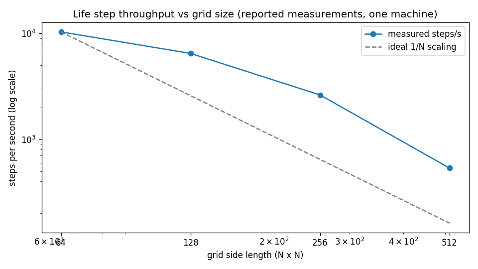
Each doubling quadruples the cells, but time per step grows only 1.5× from 64 to 128 and 2.5× from 128 to 256, because fixed per-step overhead dominates small grids. From 256 to 512 it grows 4.9×, slightly worse than proportional. That is what leaving cache-friendly sizes can look like, though this chapter does not test that explanation. The curve, not any single number, is the benchmark: it shows where this implementation stops scaling and what the next optimization must attack.
If doubling width and height gives roughly four times the work, that is expected for a local 2D update.
If runtime grows much faster, something else is happening. Measure; do not guess which.
Separate the phases
A step often contains several operations:
neighborhood construction
rule evaluation
conflict resolution
state update
measurement
rendering
Time them separately.
start = perf_counter()
neighbors = compute_neighbors(state)
t_neighbors = perf_counter() - start

start = perf_counter()
next_state = apply_rule(state, neighbors)
t_rule = perf_counter() - start
This prevents us from optimizing the wrong layer.
Rendering can dominate
A surprisingly common mistake is benchmarking simulation and visualization together.
for _ in range(1000):
    state = step(state)
    plt.imshow(state)
    plt.pause(0.01)
This measures a graphics loop as much as it measures the automaton.
For simulation benchmarks:
disable plotting
avoid disk writes
avoid animation encoding
avoid debug logging
Then benchmark visualization separately.
Memory matters too
Fast code that allocates huge temporary arrays may fail at realistic sizes.
For a (2048, 2048) float32 field:
bytes_used = 2048 * 2048 * 4
print(bytes_used / 1024**2, "MiB")
(16.0 MiB for one field.)
Now multiply that by:
current state
next state
neighbor accumulators
kernel buffers
hidden channels
batch dimension
Performance is often a memory problem before it is an arithmetic problem.
Benchmark correctness with speed
Every optimization should preserve a reference implementation.
expected = slow_step(state)
actual = fast_step(state)

assert np.array_equal(expected, actual)
For floating-point systems:
assert np.allclose(expected, actual, atol=1e-6)
A faster wrong automaton is not an optimization.
faster
  ≠ better model

asymptotic advantage
  ≠ faster at every problem size
Record benchmark metadata
Do not save only:
523 steps/s
Save:
implementation
commit
Python version
NumPy/PyTorch version
device
grid dimensions
channels
steps
seed
elapsed time
Now benchmark results become evidence rather than anecdotes.
The engineering lesson
Performance work should follow the same philosophy we used throughout the book:
observe
measure
form a hypothesis
change one thing
measure again
In the next chapter we will attack one of the most common bottlenecks directly: Python loops over cells.
Research
Python documentation:
time— Time access and conversions. The exact semantics behind this chapter’s methodology:perf_counteris the highest-resolution monotonic clock for measuring short durations (reference point undefined — only differences are meaningful). Read before building any timing harness. https://docs.python.org/3/library/time.htmlPyTorch documentation:
torch.cuda(CUDA semantics). Why warmup runs and phase separation matter on accelerators: kernel launches are asynchronous, allocation is lazy, and compilation happens once — the documented execution model that makes naive wall-clock loops lie. Essential background for the GPU chapter next. https://docs.pytorch.org/docs/stable/cuda.html