Damage, Robustness and Persistence
A pattern that survives in perfect conditions is only the beginning.
A stronger artificial-life question is:
What happens when the pattern is disturbed?
We can turn that into an experiment.
Define damage explicitly
Start with a rectangular ablation:
def damage_rectangle(state, y0, y1, x0, x1):
    damaged = state.copy()
    damaged[..., y0:y1, x0:x1] = 0.0
    return damaged
For a single-channel state:
damaged = damage_rectangle(state, 55, 70, 55, 70)
For multi-channel state, the ellipsis damages all channels in the same spatial region.
Compare damaged and undamaged controls
Always keep a control run:
control = state.copy()
damaged = damage_rectangle(state, 55, 70, 55, 70)

for _ in range(500):
    control = lenia_step(control, kernel_f, config)
    damaged = lenia_step(damaged, kernel_f, config)
Without the control, we might mistake ordinary evolution for damage response.
Measure recovery of mass
def relative_mass(state, reference):
    return float(state.sum() / max(reference.sum(), 1e-12))
Track:
immediately after damage
100 steps later
500 steps later
Mass recovery alone does not prove morphological recovery, but it is one useful signal.
A worked example on the reference configuration, ablating 26% of mass with a control run alongside: relative mass recovers 0.76 → 1.00 within 50 steps. Mass alone would declare victory — the shape measurements below refuse to. The full protocol as a diagram, with the comparison that matters made explicit:
    flowchart LR
    S[reference state] --> C[control rollout]
    S --> D[damage: ablation/noise/params]
    D --> R[recovery rollout]
    C --> M[compare: mass ratio + aligned IoU]
    R --> M
Each robustness metric answers a different question — and each can mislead alone:
| Metric | Captures | Falsely suggests when alone |
|---|---|---|
| relative mass | material return | morphology restored |
| raw IoU | pixel overlap | recovery (confounds motion) |
| aligned IoU | shape similarity modulo drift | exact state return |
| recovery time | speed back over threshold | quality of the endpoint |
Compare shape
Threshold the field:
def binary_mask(state, threshold=0.05):
    return state > threshold
Then use intersection-over-union:
def iou(a, b):
    a = binary_mask(a)
    b = binary_mask(b)

    intersection = np.logical_and(a, b).sum()
    union = np.logical_or(a, b).sum()

    if union == 0:
        return 1.0

    return float(intersection / union)
For moving organisms, direct pixel alignment is unfair.
We may need translation alignment before comparing shape.
In the same worked example, center-of-mass-aligned IoU moves 0.34 → 0.71 → 0.42 → 0.67 over 400 steps — partial, fluctuating, never restored. Mass recovered; morphology did not. Both trajectories together, from the same runs:
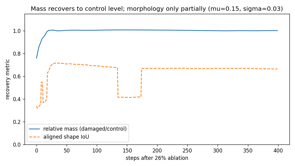
That split is the chapter’s central empirical lesson, and it is why no screenshot here is allowed to claim “regeneration.”
Align by center of mass
def shift_to_center(state):
    centre = center_of_mass(state)
    if centre is None:
        return state.copy()

    target_y = state.shape[-2] // 2
    target_x = state.shape[-1] // 2

    y, x = centre
    dy = int(round(target_y - y))
    dx = int(round(target_x - x))

    return np.roll(np.roll(state, dy, axis=-2), dx, axis=-1)
Then compare aligned states.
This separates:
shape changed
from:
shape merely moved
Noise perturbations
Damage does not have to delete a chunk.
Add noise:
def add_noise(state, amount=0.05, seed=42):
    rng = np.random.default_rng(seed)
    noise = rng.normal(0.0, amount, size=state.shape)
    return np.clip(state + noise, 0.0, 1.0)
Or randomly erase cells:
def dropout_damage(state, probability=0.1, seed=42):
    rng = np.random.default_rng(seed)
    keep = rng.random(state.shape[-2:]) > probability
    return state * keep
Different perturbations test different forms of robustness.
Parameter perturbations
The environment itself can change.
For example:
perturbed = LeniaConfig(
    radius=config.radius,
    ring_center=config.ring_center,
    ring_width=config.ring_width,
    mu=config.mu + 0.005,
    sigma=config.sigma,
    dt=config.dt,
)
Ask whether the organism still persists.
This distinguishes a broad stable basin from an exact brittle parameter point.
A robustness matrix
Run many perturbation levels:
damage fraction:  0%  10%  20%  30%  40%
noise level:       0  .01  .03  .05  .10
parameter shift:   0  .002 .005 .010 .020
For each combination record:
survival
recovery time
final mass ratio
aligned shape similarity
sustained activity
Now robustness becomes a surface, not a yes/no anecdote.
Define recovery time
def recovery_time(simulator, damaged, reference_shape, threshold=0.8, max_steps=1000):
    state = damaged.copy()

    for step_index in range(max_steps):
        state = simulator(state)
        aligned = shift_to_center(state)

        if iou(aligned, reference_shape) >= threshold:
            return step_index

    return None
The exact metric depends on the pattern, but the experimental structure is reusable. (None — never reaching threshold — is a result, distinguishing slow recovery from non-recovery the way tail activity distinguished transient from sustained dynamics.)
Robustness is not regeneration
Be careful with language.
A pattern might:
survive damage while staying deformed
or:
regrow mass but not original morphology
or:
return to a close version of its previous form
Those are different outcomes — and the worked example above landed squarely in the middle one.
Use the evidence to decide which claim is justified:
persistence after damage
  ≠ regeneration

return to similar morphology
  ≠ exact state recovery

robustness
  ≠ adaptation
Collisions are perturbations too
Place two structures near each other.
Possible outcomes:
annihilation
fusion
scattering
capture
stable coexistence
fragmentation
Track both morphology and mass through the event.
Collision experiments can expose dynamics invisible in isolated runs.
Robustness becomes a search objective
Instead of selecting candidates only for survival, evaluate them under a perturbation suite — built only from tools defined above (rectangular ablation, noise injection, mass and IoU tracking). The first scorer measures mass recovery only, and is named accordingly:
def mass_recovery_score(final, kernel_f, config, perturbations, steps=300):
    scores = []

    for perturb in perturbations:
        state = perturb(final.copy())

        for _ in range(steps):
            state = lenia_step(state, kernel_f, config)

        scores.append(relative_mass(state, final))

    return float(np.mean(scores))
with perturbations a list of callables such as damage_rectangle and add_noise partials. No undefined machinery: every piece ran earlier in this chapter.
This is intentionally a screening metric, not a robustness verdict. Mass ratio alone would have scored the worked example as a full recovery. Morphology is a separate criterion, measured with iou(shift_to_center(state), shift_to_center(final)) and reported next to the mass score. The two are not collapsed into one number, because this book has no justified weighting between them.
Now search can explicitly seek systems whose mass survives damage, and report separately whether their shape does.
A deeper limitation remains
Ordinary Lenia can create and remove local state through the growth function:
A(t + dt) = clip(A(t) + dt * G(U))
Total mass is not conserved.
That makes beautiful self-organizing dynamics possible, but it also means growth can appear locally without material being transported from somewhere else.
What happens if we impose a stronger physical-style constraint?
In the next chapter we will examine Flow-Lenia, where the update is reformulated around transport and mass conservation, and see why that changes the possibilities for interacting artificial organisms.
Research
Chan, B. W.-C. — Lenia: Biology of Artificial Life (Complex Systems 28(3), 2019). The persistence discussion this chapter operationalizes: what it means for a fuzzy, quasi-periodic pattern to survive, and the plasticity limits of that survival. The mass/shape split measured here is the quantitative form of Chan’s qualitative persistence analysis. https://arxiv.org/html/1812.05433v3
Berto, F. & Tagliabue, J. — Cellular Automata (Stanford Encyclopedia of Philosophy). The methodological backing for damage-as-probe: where analysis cannot predict the evolution, controlled perturbation with recorded context is the empirical method — the same justification that carried the discrete sensitivity chapter, now on continuous fields. https://plato.stanford.edu/entries/cellular-automata/