Sensitivity to Initial Conditions
Change one cell.
Then run the same rule twice.
If the two futures remain almost identical, the rule is insensitive to that perturbation.
If the difference spreads, the rule amplifies local uncertainty.
That is one of the cleanest experiments we can perform on a cellular automaton.
One language note up front: this chapter says “sensitive” and “irregular,” never “chaotic” in the formal dynamical-systems sense. Whether any cellular automaton earns that stronger word is a classification question for the next chapter, which owns the class vocabulary.
Create two nearby initial states
import numpy as np

width = 201
base = np.zeros(width, dtype=np.uint8)
base[width // 2] = 1

perturbed = base.copy()
perturbed[width // 2 + 1] ^= 1
The two states differ by exactly one bit.
Hamming distance
Measure the fraction of positions that differ:
def hamming_fraction(a, b):
    return float(np.mean(a != b))
At time zero:
hamming_fraction(base, perturbed)
# about 1 / 201
(Verified: exactly 1/201 ≈ 0.0050.)
Now evolve both worlds with the same rule.
Divergence curve
def divergence_curve(history_a, history_b):
    return np.array([
        hamming_fraction(a, b)
        for a, b in zip(history_a, history_b)
    ])
Plot it over time. The experiment design behind the curve:
    flowchart LR
    B[base initial state] --> RB[run rule N steps]
    P[one-bit perturbation] --> RP[run same rule N steps]
    RB --> H[Hamming distance per step]
    RP --> H
    H --> D[divergence curve]
Different rules produce very different shapes:
perturbation disappears
perturbation stays localized
perturbation spreads linearly
perturbation rapidly contaminates much of the world
(Verified on Rule 30: 0.005 → 0.42 over 200 generations — two orders of magnitude of amplification from one bit.)
Three observables, three questions — none of them chaos by itself:
| Observable | Definition | Shows | Saturates at |
|---|---|---|---|
| Hamming fraction | differing cells / width | damage extent | 1.0 (total disagreement) |
| difference width | rightmost − leftmost differing cell | spread speed | world size (geometry, not dynamics) |
| trial mean | average final Hamming over seeds | typical sensitivity | 1.0 at most; ≈ 0.5 once the two runs are statistically unrelated |
Measured on one-bit perturbations (width 201, 200 generations), four rules separate cleanly by two orders of magnitude:
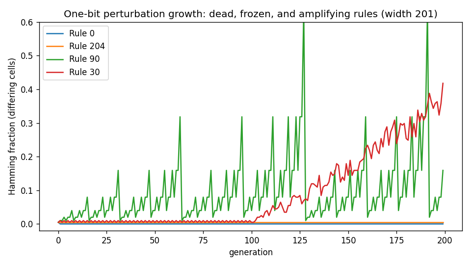
Rule 0 erases the perturbation entirely; Rule 204 freezes it in place (0.005 — the single flipped cell, forever); Rule 90 spreads it partially (0.16); Rule 30 amplifies it toward half the world (0.42). Sensitivity here is a measured spectrum, not a synonym for chaos — and the flat lines are as informative as the rising one.
The difference field
Instead of reducing everything to one number, visualize where the runs differ:
difference = history_a ^ history_b
For binary states, XOR gives us a complete perturbation map.
This can reveal a causal cone spreading away from the changed cell.
A spreading-speed estimate
Track the leftmost and rightmost differing cells:
def difference_width(a, b):
    positions = np.flatnonzero(a != b)
    if len(positions) == 0:
        return 0
    return int(positions[-1] - positions[0] + 1)
Run this at each time step to estimate how quickly perturbations expand.
The neighborhood radius imposes a maximum propagation speed, so cellular automata make causal limits explicit. On a finite ring the width saturates at the world size (verified: Rule 30 reaches the full 201-cell width) — saturation is a property of the experiment’s geometry, not proof of anything about the rule’s infinite-lattice behavior.
Repeat the experiment
One perturbation is not enough.
Run each trial from an explicit initial array with Chapter 4’s run_from_state — the runner that accepts arbitrary starts, unlike the rule-number runner which builds its own:
def sensitivity_trials(rule_number, trials=50, width=201, generations=200):
    scores = []
    rng = np.random.default_rng(42)

    for _ in range(trials):
        base = rng.integers(0, 2, size=width, dtype=np.uint8)
        changed = base.copy()
        i = rng.integers(width)
        changed[i] ^= 1

        a = run_from_state(base, rule_number, generations)
        b = run_from_state(changed, rule_number, generations)

        scores.append(float(np.mean(a[-1] != b[-1])))

    return float(np.mean(scores))
Now sensitivity becomes a property we can estimate statistically. (Verified: Rule 0 → 0.0, Rule 204 → ≈0.005, Rule 30 → ≈0.50 — the estimator separates dead, frozen, and amplifying rules by two orders of magnitude.)
Sensitivity is not automatically useful
Extreme sensitivity can mean irregular noise.
Very low sensitivity can mean a frozen system.
Again, the interesting regime may lie between extremes:
perturbations matter
but structure survives
That is particularly relevant later when we study artificial-life systems that should respond to damage without dissolving into randomness.
Robustness is the complementary question
Sensitivity asks:
How much does a small change alter the future?
Robustness asks:
Can the system recover or preserve useful structure despite a disturbance?
Those are related but not identical.
A neural cellular automaton that regrows after damage can be locally sensitive while globally robust.
We will return to that distinction later.
Next: classification
We now measure:
- density,
- activity,
- spatial variation,
- entropy,
- recurrence,
- and sensitivity.
The next question is whether these measurements can help organize rules into broad behavioral families instead of relying only on visual intuition.
Research
Zenil, H. & Martinez, G. J. — Cellular Automata (Scholarpedia). The methodology reference for this entire chapter: sensitivity studies via controlled perturbations, Hamming distance on finite configurations, damage-spreading and Lyapunov-like measures — with interpretation explicitly conditioned on metric, initial-condition distribution, and whether spread counts sites or speed. http://www.scholarpedia.org/article/Cellular_automata
Berto, F. & Tagliabue, J. — Cellular Automata (Stanford Encyclopedia of Philosophy). Grounds why the experiment matters: where prediction by analysis fails, perturbation response is the empirical probe — and the Edge-of-Chaos discussion there is the careful version of this chapter’s between-extremes intuition, with the aggregate-statistics caveats included. https://plato.stanford.edu/entries/cellular-automata/