Neural Cellular Automata for Pathfinding
Until now our neural cellular automata have learned to make and maintain shapes.
Now we will ask them to compute something.
Given:
walls
start
finish
can a shared local update rule discover a path?
This is an unusually good task for an NCA because classical pathfinding already has a local interpretation — and because recent work (Earle et al., 2023) has shown both hand-coded and learned BFS/DFS inside the NCA framework, with generalization tested on harder distributions. That paper is this chapter’s running reference: it shows the task is learnable in that setup and sets the evaluation standard.
Breadth-first search expands a frontier:
start
  ↓
nearby reachable cells
  ↓
next layer of reachable cells
  ↓
...
  ↓
goal
That has the same shape as information propagating through a cellular system.
Represent the maze as channels
Instead of one integer grid, keep semantics separate:
channel 0 = wall mask
channel 1 = start mask
channel 2 = goal mask
channel 3 = predicted distance-to-goal field (the first training target, below)
channel 4 = predicted path field (optional)
channels 5+ = hidden state
In PyTorch:
import torch

CHANNELS = 16


def make_state(walls, start, goal):
    h, w = walls.shape
    state = torch.zeros(1, CHANNELS, h, w)
    state[:, 0] = torch.as_tensor(walls, dtype=torch.float32)
    state[:, 1] = torch.as_tensor(start, dtype=torch.float32)
    state[:, 2] = torch.as_tensor(goal, dtype=torch.float32)
    return state
The first three channels are immutable problem inputs.
The other channels are working state.
Preserve the maze while updating state
Our learned rule should not rewrite the walls.
def clamp_inputs(next_state, original_state):
    next_state[:, :3] = original_state[:, :3]
    return next_state
That gives the model a stable environment while its hidden channels evolve.
A wavefront is already local computation
Classical BFS can be expressed as repeated local propagation.
Suppose frontier marks cells reached on the previous step.
import torch.nn.functional as F

CROSS = torch.tensor(
    [[0.0, 1.0, 0.0],
     [1.0, 1.0, 1.0],
     [0.0, 1.0, 0.0]]
)[None, None]


def expand(frontier, blocked):
    neighbors = F.conv2d(frontier, CROSS, padding=1)
    reachable = (neighbors > 0).float()
    return reachable * (1.0 - blocked)
(Verified: a wavefront expands around a wall segment correctly, one neighborhood per step.)
Repeated expansion spreads information one local neighborhood at a time.
An NCA does not need to invent locality.
It needs to learn what local information should propagate and how to store enough history to reconstruct a useful solution. The referenced paper hand-codes exactly this wavefront as an NCA first — then trains networks to discover equivalents, which is the order this chapter follows.
Train on distance-to-goal first
Asking for a thin exact path immediately is difficult.
A smoother training target is a distance field.
For every reachable cell, precompute its shortest-path distance to the goal with BFS.
Normalize it:
0.0 = goal
1.0 = farthest reachable cell
Then train one output channel to reproduce this field.
def distance_loss(state, target_distance, reachable_mask):
    prediction = state[:, 3:4]
    error = (prediction - target_distance).pow(2)
    return (error * reachable_mask).sum() / reachable_mask.sum().clamp_min(1)
Why is this useful?
Because a shortest path can later be recovered by descending the distance field.
Instead of learning:
which exact one-cell-wide route should I draw?
we first learn:
how far is each location from the goal?
That is a more local, redundant representation.
Roll out until information has time to travel
A maze cell cannot instantly know about a goal forty cells away.
With a radius-one neighborhood, information can move only a limited distance per update.
So training must respect the computational diameter of the problem.
Chapter 38’s rollout gains its maze form here — same word, clamped variant, since inputs must survive execution:
def rollout_frozen(model, state, steps, frozen_inputs):
    for _ in range(steps):
        state = model(state)
        state = clamp_inputs(state, frozen_inputs)
    return state
For a 32×32 maze we might sample:
steps = torch.randint(32, 65, ()).item()
For larger mazes, allow longer rollouts.
This is not merely a training hyperparameter.
Iteration count is computational depth.
Extract a path by local descent
Once a distance-like field exists, path extraction can be completely deterministic.
def descend_path(distance, start, goal, walls):
    y, x = start
    path = [(y, x)]

    for _ in range(distance.size):
        if (y, x) == goal:
            break

        choices = []
        for dy, dx in [(-1, 0), (1, 0), (0, -1), (0, 1)]:
            ny, nx = y + dy, x + dx
            if 0 <= ny < distance.shape[0] and 0 <= nx < distance.shape[1]:
                if not walls[ny, nx]:
                    choices.append((distance[ny, nx], ny, nx))

        if not choices:
            break

        _, y, x = min(choices)
        path.append((y, x))

    return path
(Verified on a walled test maze: valid start-to-goal route recovered by greedy descent.)
The three views side by side — problem, teacher signal, decoded solution — on a 28×28 maze with a 46-step optimal route:
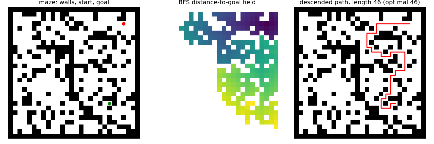
This deliberately separates learned propagation from classical decoding:
    flowchart LR
    W[walls + start + goal] --> F[local wave expansion]
    F --> D[distance field]
    D --> G[greedy descent]
    G --> P[path]
    D --> B[compare vs BFS baseline]
    P --> B
learn distributed value propagation
            ↓
use a simple deterministic decoder
We do not force the NCA to learn machinery that ordinary code already handles reliably. Component responsibilities, with the locality each one is allowed:
| Component | Role | Information scope | Verified |
|---|---|---|---|
| wave expansion | propagate reachability one neighborhood/step | strictly local | expands around walls correctly |
| distance field | per-cell goal distance | global via iteration | detours match BFS exactly |
| greedy descent | follow decreasing distance | local reads, global result | valid route on test maze |
| BFS baseline | ground truth + comparison | omniscient (not local) | optimal distances, by construction |
Compare against BFS
The baseline is not optional.
For every test maze record:
BFS reachable?
BFS shortest distance
NCA reachable prediction
NCA extracted path length
NCA valid path?
NCA excess path length
A useful metric is:
path_ratio = nca_path_length / bfs_path_length
with 1.0 meaning shortest-path performance.
Also measure outright failures separately.
A mean ratio that ignores unsolved mazes can be badly misleading.
Why learn BFS-like computation at all?
For ordinary mazes, you should simply use BFS, Dijkstra or A*.
They are explicit, efficient and exact.
The purpose of this experiment is different.
We want to discover whether a single shared local learned rule can acquire an iterative algorithm whose computation scales across a grid.
That makes pathfinding a laboratory for:
algorithmic learning
local communication
recurrent computation
generalization across spatial size
hidden-state analysis
The critical test is not the training maze
A network can memorize distributions in subtle ways.
So the important experiment begins after training.
The next chapter builds the maze training system. The chapter after it trains on small mazes and evaluates on larger, denser and structurally different mazes.
That will tell us whether the NCA learned a transferable local procedure or merely adapted to the geometry of its training set.
Research
Earle, S., Yildiz, O., Togelius, J. & Hegde, C. — Pathfinding Neural Cellular Automata (2023). The paper this chapter tracks: hand-coded BFS/DFS NCAs proving the framework can express classical search, learned variants trained from scratch (including diameter computation with strong generalization), and adversarially evolved mazes improving out-of-distribution robustness. Read before claiming any maze result is novel. https://arxiv.org/abs/2301.06820
Mordvintsev, A., Randazzo, E., Niklasson, E. & Levin, M. — Growing Neural Cellular Automata (Distill, 2020). The architectural substrate (shared local rule, hidden state, pool training) this chapter repurposes from morphogenesis to algorithmic computation. https://doi.org/10.23915/distill.00023