Use FFTs for Large Neighborhoods
Small local neighborhoods are cheap to evaluate directly.
Large smooth kernels are different.
Lenia taught us that a neighborhood may cover dozens of cells in every direction. At that scale, direct convolution can become expensive.
The Fourier transform gives us another route — provided the kernel is centered correctly, which is where the FFT bug this book had to fix lived.
Convolution becomes multiplication
For periodic domains:
convolution in space
        ↕
multiplication in frequency
So instead of sliding a large kernel over every location, we can transform both arrays, multiply them, and transform back.
But the kernel’s center must sit at the array origin first. The naive version below is wrong for the book’s own centered kernels — it treats index (0, 0) as the center and silently shifts the whole field:
def fft_convolve_naive(state, kernel):
    return np.fft.ifft2(
        np.fft.fft2(state) * np.fft.fft2(kernel, state.shape)
    ).real
Measured against the direct reference: maximum error 0.37 on a 3×3 kernel, 0.085 on a radius-13 ring. Not tolerance noise — a shifted answer. Similarly, ifftshift applied to the small kernel before padding misplaces wrapped elements (measured error 0.37/0.067): centering must happen at full array size. The correct construction is the one Chapters 29 and 31 already own — pad first, then roll the center to the origin:
import numpy as np


def centered_kernel_fft(kernel, shape):
    padded = np.zeros(shape, dtype=np.float64)
    kh, kw = kernel.shape
    padded[:kh, :kw] = kernel
    padded = np.roll(padded, -(kh // 2), axis=0)
    padded = np.roll(padded, -(kw // 2), axis=1)
    return np.fft.fft2(padded)
(Verified: maximum disagreement with direct convolution ≈ 4e-16 across radii 3, 7, and 15. Same function as kernel_fft — one owner, referenced here, not redefined. And note the parentheses again: -(kh // 2), never -kh // 2.)
Precompute static kernels
If the kernel does not change during a rollout, do not transform it every step.
kernel_f = centered_kernel_fft(kernel, state.shape)


def fft_backed_step(state, kernel_f, update_fn):
    field = np.fft.ifft2(np.fft.fft2(state) * kernel_f).real
    return update_fn(state, field)
(Named distinctly from every discrete step in the book — the FFT-backed neighborhood step takes a precomputed transform plus an update function, a different contract wearing an honest name.)
This turns repeated neighborhood evaluation into:
FFT(state)
pointwise multiply
inverse FFT
When does FFT win?
Two routes, one correct destination — and two documented ways to get the centering wrong:
    flowchart LR
    K[centered kernel] --> D[direct: shift-multiply-add]
    K --> F[pad, roll center to origin, FFT, multiply, IFFT]
    D --> S[same periodic field]
    F --> S
    W[naive fft2 of raw kernel] --> X[shifted field: wrong]
    Y[ifftshift before padding] --> Z[misplaced wrap: wrong]
Not always — measured on a 256×256 grid, precomputed kernel, this machine:
| Radius | Taps | Direct | FFT | Winner |
|---|---|---|---|---|
| 1 | 9 | 0.36ms | 2.16ms | direct |
| 3 | 49 | 2.02ms | 2.01ms | tie |
| 7 | 225 | 10.15ms | 2.22ms | FFT |
| 15 | 961 | 50.72ms | 2.07ms | FFT |
| 31 | 3969 | 209.05ms | 2.26ms | FFT |
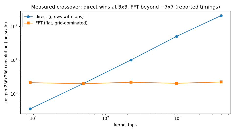
Direct cost grows with taps; FFT cost stays nearly flat (grid-dominated) while error creeps from 5e-16 to 3e-15 with kernel size — still far below any modeling tolerance, but the trend is why behavioral validation over rollouts matters more than single-step agreement. The plot shows the same numbers as the table: use whichever your eye reads faster, but neither replaces measuring on your own workload.
The crossover depends on:
grid size
kernel size
backend
batch size
CPU/GPU
precision
Measure it — on your grid, your kernel, your hardware. The table above is evidence for one configuration, not a universal constant.
Compare implementations
def compare(a, b):
    error = np.max(np.abs(a - b))
    print("max error:", error)

field_direct = periodic_convolve(state, kernel)  # Chapter 29's owner
field_fft = fft_backed_step(state, kernel_f, lambda s, f: f)
compare(field_direct, field_fft)
Boundary semantics must match.
A circular FFT convolution is naturally periodic. Comparing it with zero-padded direct convolution is comparing different models.
Multi-channel systems
For several channels and kernels, frequency-domain computation can be batched.
Conceptually:
state channel FFTs
        ↓
frequency-domain kernel mixing
        ↓
inverse FFTs
        ↓
growth/update functions
This is useful for multi-kernel Lenia and related systems.
GPU FFTs
PyTorch exposes FFT operations directly:
state_f = torch.fft.fft2(state)
kernel_f = torch.fft.fft2(centered_kernel)
field = torch.fft.ifft2(state_f * kernel_f).real
with centered_kernel built by the same pad-then-roll construction — raw fft2(kernel) carries the identical shift bug as the naive NumPy version.
Again, keep tensors on the device throughout the rollout.
Numerical differences are expected
Direct and FFT-based convolution can differ slightly because floating-point operations occur in a different order.
For continuous dynamical systems, tiny differences may grow over long rollouts.
Therefore validate at two levels:
local numerical agreement
behavioral agreement over time
The second is often more important than expecting bit-identical trajectories.
FFT is asymptotically faster
  ≠ faster at small kernels

numerically close
  ≠ bit-identical

FFT convolution
  ≠ linear convolution unless padding semantics match
Choose the algorithm from the structure
We now have three broad neighborhood strategies:
small stencil          → shifts/slices/direct convolution
learned local kernels  → standard tensor convolution
large periodic kernels → FFT convolution
A reusable cellular-automata system should make those choices explicit rather than burying them inside each chapter’s code.
That is what we build next.
Research
NumPy documentation: Discrete Fourier Transform (
numpy.fft). The exact machinery behind this chapter: the convolution theorem, real-inputrfftvariants worth reaching for on real fields, and thefftshift/ifftshifthelpers — with the caveat, demonstrated above, that shifting must happen at full array size to mean circular convolution. https://numpy.org/doc/stable/reference/routines.fft.htmlPython documentation:
time— Time access and conversions. The crossover table stands onperf_counterdifferences with warmup separated; without that discipline a “crossover point” is an anecdote about one machine’s mood. https://docs.python.org/3/library/time.html