Conway's Game of Life
The previous chapter ended on a limit of one dimension: time supplies the second visual axis, but structures cannot move inside the world. In two dimensions they can. Conway’s Game of Life is one of the cleanest examples of intricate two-dimensional behavior emerging from a tiny local rule.
John Conway devised it in 1970; Martin Gardner’s October 1970 Scientific American column introduced it to a wide audience and triggered the volunteer zoology of patterns — still lifes, oscillators, spaceships — that made Life the most studied cellular automaton in history.
The world is a grid of dead and live cells.
Each cell sees its eight surrounding neighbors.
Then four ideas decide the next generation:
underpopulation
survival
overpopulation
birth
The standard rule is usually written B3/S23:
- a dead cell is born with exactly 3 live neighbors,
- a live cell survives with 2 or 3 live neighbors.
Everything else becomes or remains dead. As a decision flow, with n live neighbors:
    flowchart TD
    A[cell with n live neighbors] --> B{currently alive?}
    B -->|no| C{n == 3?}
    B -->|yes| D{n == 2 or n == 3?}
    C -->|yes| E[born: becomes alive]
    C -->|no| F[stays dead]
    D -->|yes| G[survives: stays alive]
    D -->|no| H[dies: underpopulation or overpopulation]
The same machinery, a richer neighborhood
It helps to place Life next to the elementary rules before building it:
Elementary CA:
  1D line
  2 states
  radius-1 neighborhood (self + 2 neighbors)
  8 neighborhood configurations -> 256 tables

Life:
  2D grid
  2 states
  Moore neighborhood (self + 8 neighbors)
  512 neighborhood configurations
The conceptual machinery is identical — lattice, finite states, local update, synchronous parallel step. What changed is only the size of the lookup: each cell’s fate now depends on nine bits rather than three. B3/S23 is one point in that 512-row space, picked out by a birth set and a survival set rather than an arbitrary table. Rules of this birth/survival form are called Life-like; the next chapters will explore its neighbors, but this chapter stays with B3/S23 itself.
Represent the grid
import numpy as np

grid = np.zeros((40, 60), dtype=np.uint8)
Seed a simple three-cell line:
grid[20, 29:32] = 1
That pattern is the blinker.
Count neighbors with array shifts
We can count all eight neighbors using np.roll:
def neighbor_count(grid):
    total = np.zeros_like(grid, dtype=np.uint8)

    for dy in (-1, 0, 1):
        for dx in (-1, 0, 1):
            if dx == 0 and dy == 0:
                continue
            total += np.roll(np.roll(grid, dy, axis=0), dx, axis=1)

    return total
This gives periodic boundaries: the top connects to the bottom and the left edge connects to the right. Our 40×60 world is a torus, not an unbounded plane.
That is a modeling choice worth naming. The classic Life results — gliders traveling indefinitely, glider guns firing forever, universal constructions — assume an infinite lattice. On our torus a glider eventually wraps around and collides with its own trail. Finite boards are honest laboratories as long as we remember they are finite; the next chapter’s pattern library will need steady or well-separated configurations precisely because the board has edges only in the topological sense.
Now implement B3/S23:
def life_step(grid):
    n = neighbor_count(grid)

    born = (grid == 0) & (n == 3)
    survive = (grid == 1) & ((n == 2) | (n == 3))

    return (born | survive).astype(np.uint8)
That is the complete Game of Life rule.
The same synchronous-update discipline from our one-dimensional automata still applies: every birth and death is calculated from the same current generation.
Watch an oscillator
for generation in range(4):
    print(f"generation {generation}")
    print(grid[18:23, 27:34])
    grid = life_step(grid)
The blinker alternates between horizontal and vertical states. (Verified: identical after two steps, different after one — a genuine period-2 cycle.)
So we have found our first repeating cycle:
state A -> state B -> state A -> ...
Seed a glider
glider = np.array([
    [0, 1, 0],
    [0, 0, 1],
    [1, 1, 1],
], dtype=np.uint8)

grid = np.zeros((60, 80), dtype=np.uint8)
grid[5:8, 5:8] = glider
Repeated Life updates cause the pattern to reproduce its shape at an offset.
The canonical static figure shows four phases of that motion:
python scripts/figures/cellular-automata/part01_foundations.py 05
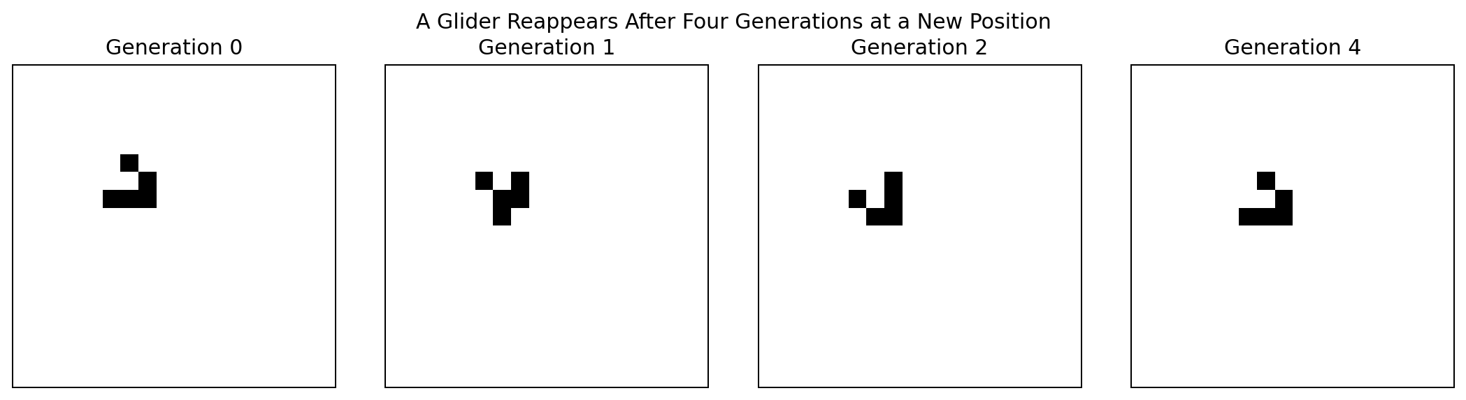
After four generations the glider has the same orientation but is shifted one cell diagonally. (Verified in code: the 3×3 patch reappears exactly, offset by (+1, +1).)
That means a local configuration has become a moving object.
No code says:
glider.move_diagonally()
Movement is an observed dynamical behavior of repeated births and deaths — not a programmed method, not evidence of agency, and not a claim that anything is alive.
Animate the simulation
import matplotlib.pyplot as plt
from matplotlib.animation import FuncAnimation

fig, ax = plt.subplots()
image = ax.imshow(grid, cmap="binary", interpolation="nearest")
ax.axis("off")


def animate_frame(_):
    global grid
    grid = life_step(grid)
    image.set_data(grid)
    return (image,)

animation = FuncAnimation(fig, animate_frame, interval=80, blit=True)
plt.show()
The animation is useful, but keep the transition function separate from rendering.
That gives us:
model -> state transition
view  -> visualization
and prevents display code from defining the simulation.
Classify patterns by behavior
Life produces several broad kinds of structure.
Still lifes
Patterns that stop changing.
Examples include blocks (verified: a 2×2 block is a fixed point of life_step) and beehives.
Oscillators
Patterns that repeat after a fixed period.
The blinker has period two.
Spaceships
Patterns that repeat after a fixed number of generations but at a translated position.
The glider is the canonical example.
Methuselahs
Small initial patterns that evolve for a surprisingly long time before settling into simpler debris.
These categories are useful because they describe dynamics, not merely shape. A block and a beehive look different but belong together; a glider and a blinker can look similar in a single snapshot but belong apart. Only two patterns are worked examples in this chapter — the blinker and the glider — because each teaches a new mechanism (cycling, translation). The rest arrive as named categories for the library we build next.
Measure population through time
def simulate_life(grid, steps):
    history = []
    state = grid.copy()

    for _ in range(steps):
        history.append(state.copy())
        state = life_step(state)

    return np.array(history)

history = simulate_life(grid, 200)
population = [state.sum() for state in history]

plt.plot(population)
plt.xlabel("generation")
plt.ylabel("live cells")
plt.show()
Population alone cannot tell us what structures exist, but it is one useful observable.
We can add:
- bounding-box size,
- number of connected components,
- period detection,
- translation detection,
- entropy,
- collision outcomes.
This is how we move from watching Life to analyzing Life.
The deeper programming lesson
A glider looks like an object.
But there is no glider object in the implementation.
There are only cells and a local update rule.
That distinction is important:
implementation ontology:
    cells + rules

observer ontology:
    gliders + blinkers + spaceships
Higher-level entities can be real and useful even when they are not primitive objects in the code.
That is one of the most important ideas in emergent systems — stated here as an observed dynamical behavior with a concrete demonstration (the verified glider translation), not as a metaphysical thesis. The book keeps the related claims separated throughout:
visually rich
  ≠ alive
  ≠ self-reproducing
  ≠ universal
Life’s patterns are visually rich: established by inspection. Nothing here is alive, nothing shown so far reproduces itself, and universality — though genuinely established for Life via constructed glider logic and explicit universal configurations — is a formal property of arranged initial conditions on an unbounded grid, whose machinery belongs to Chapter 27. This chapter establishes Life as a system where signals visibly move; the later chapter shows what those signals can be made to compute.
In the next chapter we will exploit that idea directly: we will build a small library of Life patterns, detect oscillation and movement, and treat recurring structures as data.
Research
Gardner, M. — Mathematical Games: The fantastic combinations of John Conway’s new solitaire game “Life” (Scientific American 223(4), 1970). The original popularization and the source for the early history: Conway’s rule, the first named patterns, and the conjectures that launched Life’s study. Prefer this over retold folklore for any historical claim. https://doi.org/10.1038/scientificamerican1070-120
Berto, F. & Tagliabue, J. — Cellular Automata (Stanford Encyclopedia of Philosophy), §§2.5–2.6. Places Life in the book’s conceptual frame: the B3/S23 schema on the Moore neighborhood, the glider/oscillator/eater pattern gallery as observed behavior, and the universality argument via storage, transmission, and logic-gate primitives (Berlekamp, Conway & Guy 1982) plus Rendell’s explicit Turing machine — with unpredictability grounded in the halting problem rather than in visual richness. https://plato.stanford.edu/entries/cellular-automata/
Zenil, H. & Martinez, G. J. — Cellular Automata (Scholarpedia). Verifies the technical details this chapter depends on: the Moore-neighborhood counting convention, the exact B3/S23 rule, Gardner (1970) as the introductory reference, and the qualifier that universal computation in Life requires deliberately arranged configurations rather than arising from every initial pattern. http://www.scholarpedia.org/article/Cellular_automata