Search Lenia Parameter Space
A Lenia pattern is not defined by its initial state alone.
It also lives inside a particular dynamical world.
Change the kernel or growth function slightly and the same seed may:
die
explode
freeze
oscillate
move
split
stabilize into a different morphology
So discovery has two coupled search spaces:
initial condition
      +
world parameters
Define parameter ranges
PARAM_RANGES = {
    "radius": (8, 24),
    "ring_center": (0.25, 0.75),
    "ring_width": (0.05, 0.25),
    "mu": (0.05, 0.30),
    "sigma": (0.01, 0.08),
    "dt": (0.03, 0.20),
}
These ranges are experimental choices.
They define which region of Lenia space we are willing to explore. (Chan’s maps span the same μ–σ plane among others — including the β-cube this single-ring implementation does not reach, a stated scope limit from Chapter 31.)
Each parameter’s local role — and how its failure looks, so the heatmap below reads as diagnosis rather than decoration:
| Parameter | Role | Too low | Too high |
|---|---|---|---|
| mu | preferred neighborhood density | sparse contexts starve | crowding saturates |
| sigma | tolerance width | selective to the point of death | indiscriminate flooding |
| radius | kernel scale | fine detail, small structures | coarse, slow, expensive |
| dt | integration step | sluggish convergence | instability |
Sample a configuration
def sample_config(rng):
    return LeniaConfig(
        radius=int(rng.integers(8, 25)),
        ring_center=float(rng.uniform(0.25, 0.75)),
        ring_width=float(rng.uniform(0.05, 0.25)),
        mu=float(rng.uniform(0.05, 0.30)),
        sigma=float(rng.uniform(0.01, 0.08)),
        dt=float(rng.uniform(0.03, 0.20)),
    )
A random search is not sophisticated.
But it gives us a baseline.
Never build an elaborate optimizer before measuring what random search can already find.
Evaluate configurations and seeds together
def evaluate_trial(config, seed_value, shape=(128, 128), steps=500):
    initial = random_seed(shape=shape, seed=seed_value)
    result = evaluate_seed(initial, config, steps=steps)

    return {
        "config": config,
        "seed": seed_value,
        "score": candidate_score(result),
        "result": result,
    }
Then:
rng = np.random.default_rng(1234)
trials = []

for trial_id in range(200):
    config = sample_config(rng)
    seed_value = int(rng.integers(0, 1_000_000))
    trials.append(evaluate_trial(config, seed_value))
Separate failure categories
A single low score hides useful information.
Record explicit outcomes:
def classify_outcome(result):
    final = result["final"]
    mass = final.sum()
    fraction = result["active_fraction"]
    activity = result["activity"]

    if mass < 1e-3:
        return "dead"
    if fraction > 0.8:
        return "world-filling"
    if activity < 1e-5:
        return "static"
    return "persistent-dynamic"
Now we can ask:
Which parameters tend to die?
Which explode?
Where do persistent structures cluster?
Failure becomes data.
Plot the search landscape
import matplotlib.pyplot as plt

x = [t["config"].mu for t in trials]
y = [t["config"].sigma for t in trials]
c = [t["score"] for t in trials]

plt.scatter(x, y, c=c)
plt.xlabel("mu")
plt.ylabel("sigma")
plt.colorbar(label="candidate score")
plt.show()
This is the book’s version of Chan’s μ–σ maps, which chart species distributions across growth-parameter space: a two-dimensional projection of a larger parameter space, where persistent regions — not individual champions — are the finding.
But projections can reveal regions worth exploring more densely. Measured here over a 6×5 μ–σ grid (2 seeds per cell, 150 steps, 96×96, full candidate score with real activity):
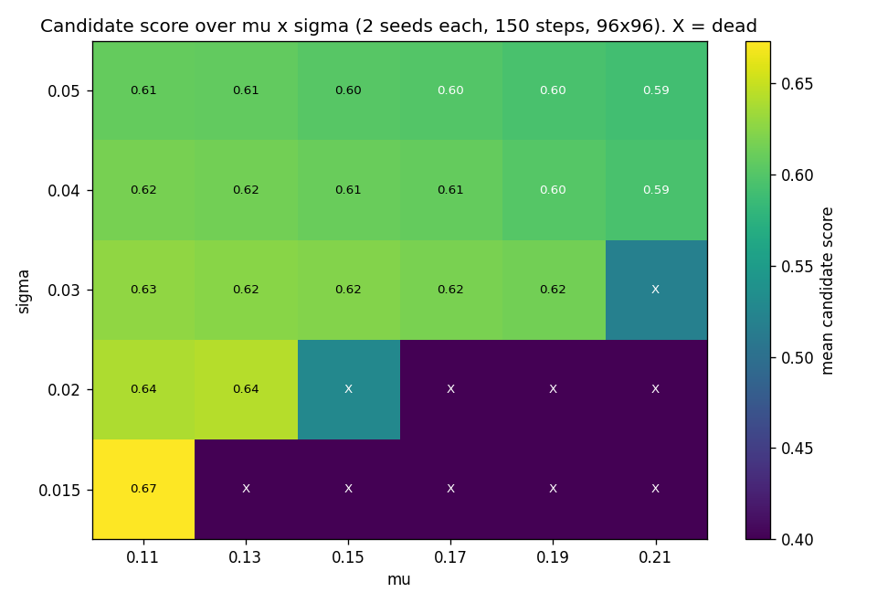
Scores run 0.40 (dead) to ~0.67 with a persistent interior around μ ≈ 0.13–0.17, σ ≥ 0.02 and extinction along the narrow-sigma border. Read it as a map of where to search, not a phase theorem — 150 steps and 2 seeds per cell resolve regimes, not boundaries.
Local refinement
Once a promising configuration appears, mutate around it:
def mutate_config(config, rng):
    return LeniaConfig(
        radius=max(3, config.radius + int(rng.integers(-2, 3))),
        ring_center=float(np.clip(config.ring_center + rng.normal(0, 0.03), 0.05, 0.95)),
        ring_width=float(np.clip(config.ring_width + rng.normal(0, 0.02), 0.01, 0.40)),
        mu=float(np.clip(config.mu + rng.normal(0, 0.015), 0.01, 0.50)),
        sigma=float(np.clip(config.sigma + rng.normal(0, 0.008), 0.005, 0.20)),
        dt=float(np.clip(config.dt + rng.normal(0, 0.01), 0.01, 0.30)),
    )
The strategy becomes:
explore broadly
      ↓
find promising region
      ↓
search locally
Robustness matters more than one lucky run
A configuration that works for one exact seed may be extremely fragile.
Evaluate multiple nearby seeds:
def robustness_score(config, seeds, steps=500):
    scores = []

    for seed_value in seeds:
        initial = random_seed(seed=seed_value)
        result = evaluate_seed(initial, config, steps=steps)
        scores.append(candidate_score(result))

    return {
        "mean": float(np.mean(scores)),
        "minimum": float(np.min(scores)),
        "std": float(np.std(scores)),
    }
A robust region should not collapse under tiny changes in initialization.
The regime test, executed on the reference configuration: shifting μ by ±0.02, widening σ by +0.02, or doubling dt all preserve persistent dynamics (masses ≈ 1785–2237) — quantitative change within qualitative persistence. But narrowing σ by 0.015 kills the pattern outright. That is the honest shape of a parameter region: robust interior, fragile borders, verified rather than asserted.
Search for niches, not just champions
The highest score may not be the most interesting result.
Imagine three candidates:
A: stationary pulsing blob
B: fast translating crescent
C: branching structure that repeatedly repairs itself
A single score may rank one highest and discard the others.
Instead maintain an archive indexed by behavioral descriptors:
speed
mass
size
activity
symmetry
oscillation period
Keep the best candidate in each region of behavior space.
This is the quality-diversity idea in practical form.
Search produces maps of possibility
A good search system does more than return one organism.
It can reveal:
stable regions
fragile borders
extinction zones
world-filling zones
mobile-pattern niches
oscillatory niches
That changes the scientific question from:
What creature did we find?
into:
What kinds of behavior are possible in this family of worlds?
Store the complete experiment table
Save every trial, not just winners.
A tabular record might contain:
trial_id
seed
radius
ring_center
ring_width
mu
sigma
dt
survival
mass
activity
active_fraction
classification
score
artifact_path
Then later analysis does not require rerunning every simulation.
The rule itself can become richer
So far one kernel produces one perception field and one growth response.
But many biological systems operate at more than one spatial scale.
We can have:
several kernels
several channels
several growth responses
cross-channel influence
That is the next major expansion — and the canonical direction: Chan’s full formulation already carries multi-shell β kernels, and multi-kernel/channel systems generalize further.
In the next chapter we will build multi-kernel and multi-channel Lenia, where a cell’s state becomes a vector again and different local fields can interact.
Research
Chan, B. W.-C. — Lenia: Biology of Artificial Life (Complex Systems 28(3), 2019). The mapping precedent for this chapter: μ–σ maps and the β-cube charting where species live in parameter space, niches and landscapes as the unit of discovery, and the stability–motility hypothesis linking persistence to movement. Run the regime test first; read the maps second. https://arxiv.org/html/1812.05433v3
Lehman, J. & Stanley, K. O. — Abandoning Objectives (Evolutionary Computation 19(2), 2011). The reason the archive is indexed by behavior rather than score: novelty in descriptor space finds what champion-chasing discards. The niches section is quality diversity argued from the book’s own candidates. https://dl.acm.org/doi/10.1162/EVCO_a_00025