Build a Predator-Prey Ecosystem
Gray-Scott, like the forest fire, transforms each cell in place.
Rule 184 moves occupancy, but in one constrained direction.
An ecosystem adds a harder problem:
organisms move
organisms reproduce
predators consume prey
several organisms may want one destination
Now local intentions can conflict.
That means update semantics become part of the model.
Separate visible kind from internal state
Start with:
0 = empty
1 = prey
2 = predator
import numpy as np

EMPTY = 0
PREY = 1
PREDATOR = 2

kind = np.zeros(
    (100, 100),
    dtype=np.uint8,
)
A richer model may need predator energy, age or reproduction state.
Do not overload one integer with every concept.
Use additional fields:
energy = np.zeros(
    kind.shape,
    dtype=np.float32,
)
Now a cell’s state is layered:
visible occupancy
+
internal organism state
This continues Chapter 8’s lesson about state as local memory — now the memory records per-organism history (energy, age) rather than just a refractory timer.
Why naive in-place movement is dangerous
Suppose two predators both target the same prey.
If we mutate the grid immediately, whichever predator happens to be processed first wins.
Then Python loop order has become part of the ecology.
Sometimes sequential updates are a deliberate model choice.
But if they are not deliberate, they are a hidden source of causality. The classic cautionary case is Huberman and Glance’s 1993 spatial-games result: outcomes that looked like discoveries about cooperation turned out to depend on synchronous updating, and introducing asynchrony changed the dynamics. Update order is never neutral scenery; it is always either a stated assumption or an uncontrolled one.
A cleaner synchronous architecture is:
current world
      ↓
propose actions
      ↓
resolve conflicting targets
      ↓
apply accepted actions
      ↓
next world
That is very close to transaction processing.
Make conflict resolution explicit
A prey movement proposal might look like:
(source, target, PREY)
Group proposals by target:
from collections import defaultdict


def resolve_targets(
    proposals,
    rng,
):
    by_target = defaultdict(list)

    for proposal in proposals:
        by_target[
            proposal[1]
        ].append(proposal)

    accepted = []

    for target, choices in by_target.items():
        choice = choices[
            rng.integers(len(choices))
        ]

        accepted.append(choice)

    return accepted
(Verified: with two proposals targeting one cell and one targeting another, exactly one winner per target is accepted.)
Now the collision policy is part of the experiment.
We could instead choose:
| Policy | Who wins a contested cell | Modeling implication |
|---|---|---|
| first proposal | loop order | fast but order-dependent — usually a bug |
| highest-energy organism | strongest claimant | merit-based, needs energy state |
| random proposal | uniform draw | neutral, seed-controlled |
| no proposal | nobody moves in | cautious, may deadlock |
| priority by species | fixed ranking | built-in asymmetry, state it openly |
Those are different models.
Give predators persistent state
A predator can lose energy every step and gain energy when it eats.
MOVE_COST = 1.0
FOOD_ENERGY = 4.0
Conceptually:
choose local action
      ↓
pay movement cost
      ↓
gain food energy if predation succeeds
      ↓
die if energy <= 0
Now the future depends on local history.
State has become memory.
Track the world and the populations separately
A spatial snapshot tells us where interactions occur.
A population curve tells us what happens globally.
Those are complementary observables.
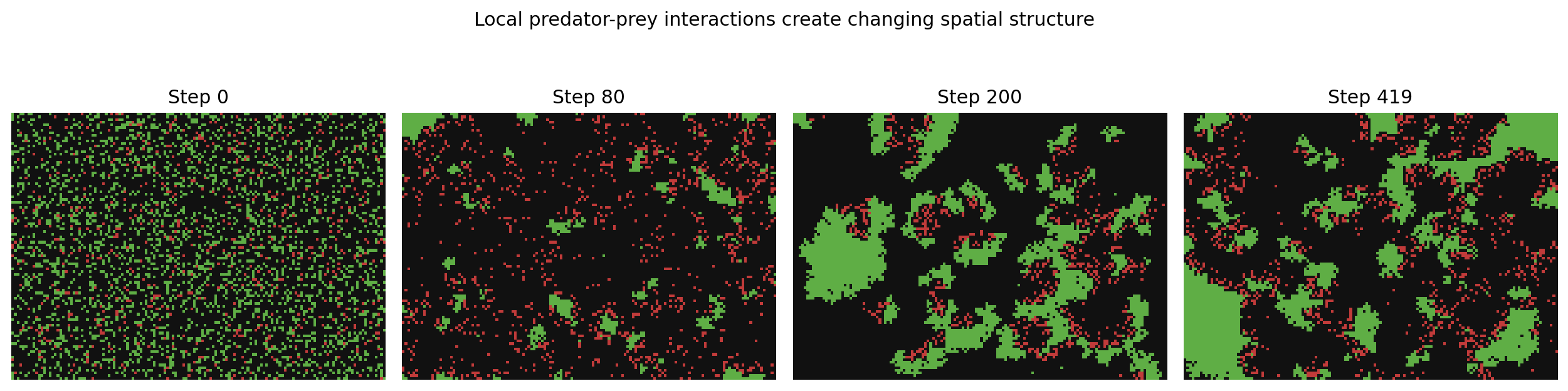
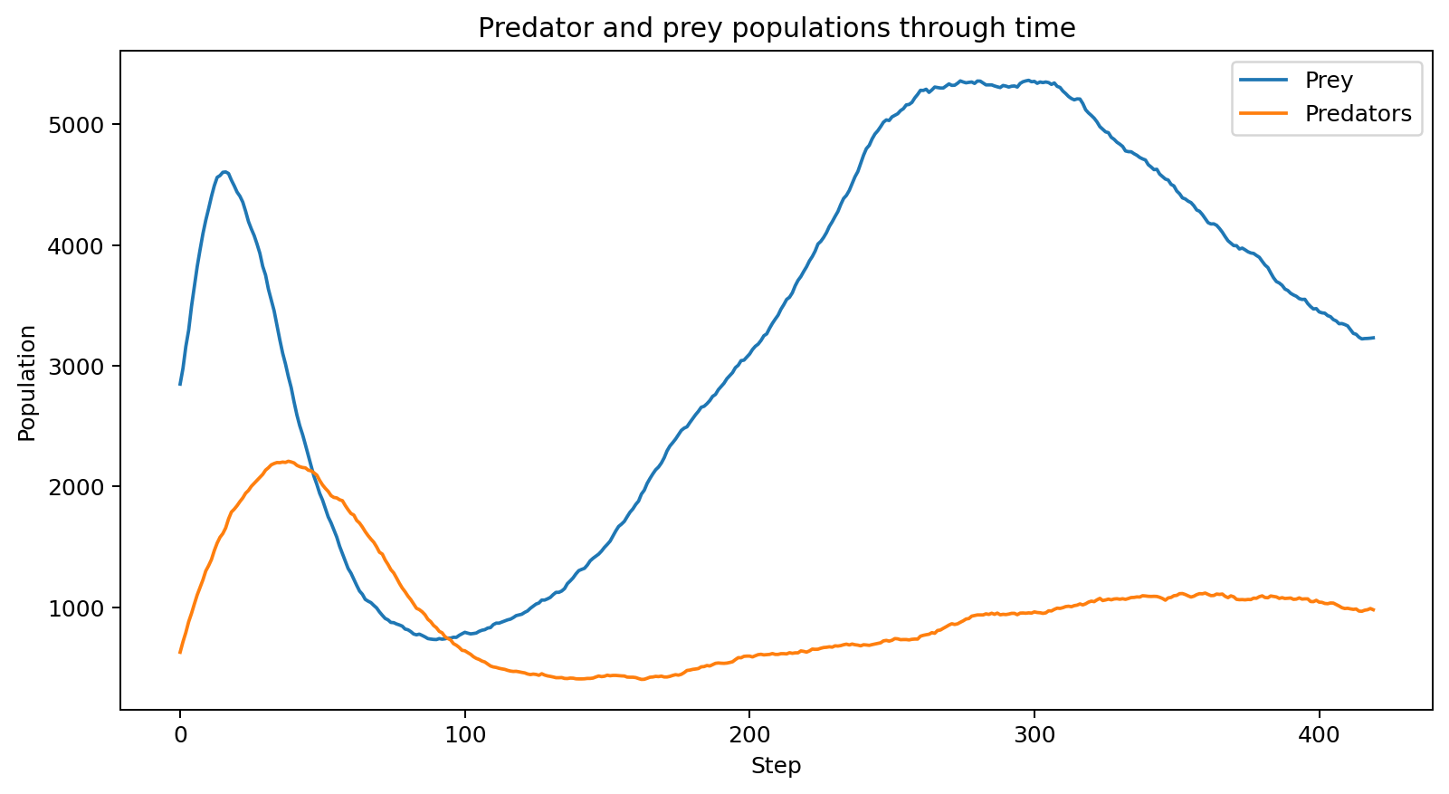
The figure generator uses a deliberately compact local predator-prey CA to visualize the population-level phenomenon.
The chapter’s propose/resolve architecture is the richer implementation pattern to use when explicit movement and target conflicts matter.
That distinction is useful:
figure model:
demonstrate spatial population dynamics

engineering model:
make agent intentions and conflicts inspectable
Stating which model produced a figure is part of honest reporting: the curves illustrate possible dynamics, not predictions of the propose/resolve system.
Oscillation is not guaranteed
It is tempting to draw this loop:
prey increase
      ↓
predators increase
      ↓
prey decrease
      ↓
predators starve
      ↓
prey recover
That mechanism can produce oscillatory population dynamics.
But not every parameter choice will.
Possible outcomes include:
prey extinction
predator extinction
both extinction
persistent coexistence
oscillation
spatial patchiness
So the existence and character of oscillation should be measured rather than assumed — with the guardrail that an observed oscillation is not yet a demonstrated stable limit cycle, and neither is ecological realism. Cycles in a toy spatial system suggest mechanisms worth testing, not predictions about real populations.
Treat hidden choices as parameters
Important choices include:
neighborhood shape
movement policy
collision resolution
predation probability
reproduction probability
energy gain
energy cost
boundary conditions
update synchrony
If those remain buried inside code, two ecosystem runs are difficult to compare meaningfully.
Make them explicit configuration.
Keep causality inspectable
When an organism disappears, we should know why.
A lightweight event record can help:
from dataclasses import dataclass


@dataclass
class Event:
    kind: str
    source: tuple[int, int] | None
    target: tuple[int, int] | None
Possible event kinds:
move
eat
birth
starve
collision_lost
Now debugging does not require reconstructing every causal decision from snapshots after the fact.
This becomes increasingly important as cellular systems start to resemble local agents.
One idea to keep
The difficult part of multi-agent cellular worlds is not merely writing more transition rules.
It is defining what simultaneous local action means.
Once several cells compete for shared resources or destinations, conflict resolution becomes part of the model.
In the next chapter we will use local updates for a different purpose: not to simulate an ongoing world, but to construct an organic cave map and then validate whether the result is actually usable.
Research
Huberman, B. A. & Glance, N. S. — Evolutionary Games and Computer Simulations (1993). The cautionary case behind this chapter’s update-semantics warning: spatial-game outcomes that looked like discoveries about cooperation depended on the synchronous update scheme, and asynchrony changed the dynamics. Read before treating any multi-agent result as scheme-independent. https://www.researchgate.net/publication/14843377_Evolutionary_Games_and_Computer_Simulations
Zenil, H. & Martinez, G. J. — Cellular Automata (Scholarpedia). Distinguishes the update-scheme relaxations this chapter navigates: non-uniform automata (rule varies by position) versus asynchronous updating (timing varies), plus stochastic local updates. Use it to name which relaxation a design actually uses. http://www.scholarpedia.org/article/Cellular_automata
Berto, F. & Tagliabue, J. — Cellular Automata (Stanford Encyclopedia of Philosophy). Covers asynchronous updating as a legitimate modeling choice (Ingerson & Buvel 1984) and the broader simulator lineage — the framing that keeps this chapter’s toy ecology a mechanism study rather than a biological claim. https://plato.stanford.edu/entries/cellular-automata/