Flow-Lenia and Mass-Conserving Artificial Life
Ordinary Lenia updates local state by adding growth:
A(t + dt) = clip(A(t) + dt × G(U))
That means state can be created in one region and destroyed in another.
For many artificial-life experiments that is perfectly acceptable.
But it leaves a major question:
What changes if local structure must reorganize existing mass instead of creating or deleting it?
Flow-Lenia — Plantec et al. (2023), “Flow-Lenia: Towards open-ended evolution in cellular automata through mass conservation and parameter localization” — explores exactly that direction through two ideas: reformulating the update around transport so mass is conserved, and embedding rule parameters as local fields rather than global constants. This chapter presents both ideas with small pedagogical models, honestly labeled as stepping stones rather than reproductions.
Why conservation changes the problem
Imagine a grid whose values represent material density.
In a non-conservative update:
0.2 -> 0.7
can happen because the growth function says so.
In a conservative model, an increase here must be balanced by movement from somewhere else.
Conceptually:
mass leaves neighboring cells
        ↓
flows through local transport
        ↓
arrives here
The total remains approximately constant:
state.sum()
before and after the update.
Start with a transport field
We can build a simple pedagogical mass-conserving model before attempting anything Flow-Lenia-specific.
Suppose every cell has a scalar density field:
import numpy as np

state = np.zeros((128, 128), dtype=np.float64)
state[48:80, 48:80] = np.random.default_rng(42).random((32, 32))
Flow-Lenia derives its transport from local perception. The toy model below is deliberately simpler: it moves mass down the gradient of the density itself.
A minimal conservative flow step
This toy demonstrates conservative local transport. It is not an implementation of the full Flow-Lenia transport mechanism.
It is a small model that makes the conservation principle explicit. Because it moves mass only down the density gradient, it behaves like diffusion: it conserves mass, but it will not sustain structures on its own.
def conservative_flow_step(state, rate=0.1):
    next_state = state.copy()

    for axis in (0, 1):
        neighbor = np.roll(state, -1, axis=axis)
        gradient = state - neighbor

        flow = rate * gradient

        next_state -= flow
        next_state += np.roll(flow, 1, axis=axis)

    return np.clip(next_state, 0.0, None)
Check total mass:
before = state.sum()
after_state = conservative_flow_step(state)
after = after_state.sum()

print(before, after, after - before)
(Verified: bit-exact conservation on the test field, drift 0.0; 200-step drift ≈ 1e-13. The clip binds only if flow drives a cell negative — on smooth fields it never does, but the guard stays because a conservation claim should be checked every run, not assumed from intent.)
Numerical details matter, but the intended invariant is clear:
mass moved
mass was not invented
Conservation gives us a testable invariant
We can write:
def assert_mass_conserved(before, after, atol=1e-9):
    assert np.isclose(before.sum(), after.sum(), atol=atol)
This is stronger than merely looking at an animation.
A conserved quantity gives the simulation a hard correctness property. Measured side by side from the same soup (96×96, 200 steps):
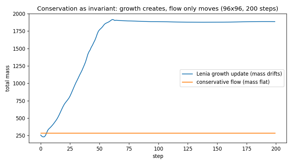
The flat line is the invariant working; the climbing line is ordinary Lenia creating mass where its growth function says so. Neither is “better” — they are different semantics, and the plot tells you which one you implemented.
From growth field to flow field
In ordinary Lenia:
local perception
      ↓
growth or decay
In a flow-based system we instead want something closer to:
    flowchart LR
    P[local perception] --> D[transport tendency: where should mass go?]
    D --> R[redistribute existing material]
    R --> N[next state: same total mass]
That is a much deeper change than replacing one equation with another.
The update semantics themselves have changed. Growth creates and destroys; flow only moves:
| Aspect | Ordinary Lenia | Flow-Lenia direction |
|---|---|---|
| state change mechanism | add growth, clip | transport existing mass |
| total mass | drifts freely | conserved (invariant) |
| rule parameters | global constants | localizable fields |
| new capability | rich pattern formation | coexistence, interaction of regimes |
Think of material as particles without particles
We still store a continuous density field.
But conceptually we can imagine each cell asking:
where should my local mass move?
The grid remains Eulerian:
fixed spatial cells
while state moves through it.
That is the aim of the flow formulation: structures that move through a fixed grid by transporting mass, without explicitly simulating millions of individual particles. The toy model above demonstrates only the conservation half of that idea.
Local parameters can become part of state
The second Flow-Lenia pillar is that rule parameters can be localized — embedded in the dynamics rather than fixed globally.
Instead of one world-wide parameter:
mu = 0.15
we can imagine a field:
mu = np.full((128, 128), 0.15)
Different regions can carry different local rule values.
Now an artificial organism can potentially carry aspects of its own update dynamics with it.
Conceptually:
matter field
parameter field
      ↓
local dynamics
This creates the possibility of several locally coherent rule regimes coexisting in one world.
A toy localized-parameter field
mu = np.full(state.shape, 0.15)
mu[40:70, 40:70] = 0.12
mu[70:100, 70:100] = 0.20
A local response function can then use:
def local_growth(u, mu_field, sigma=0.03):
    return 2.0 * np.exp(
        -((u - mu_field) ** 2) / (2 * sigma ** 2)
    ) - 1.0
(Verified: runs elementwise over fields without shape errors.)
Again, this is an explanatory stepping stone rather than a complete Flow-Lenia reproduction — the book’s vectorized form of the localized-parameter idea, not the paper’s embedded-parameter machinery.
The important conceptual shift is that rule identity no longer has to be globally fixed.
Multi-species becomes a systems question
If two structures carry different local parameters, then when they meet we must decide how parameter fields interact.
Possible mechanisms include:
mix
compete
average
remain spatially separated
inherit during redistribution
Now the model can support questions closer to ecology and evolution:
Can multiple persistent forms coexist?
Can one displace another?
Can local rule information spread?
Can new combinations appear?
Measure evolutionary activity carefully
A changing picture is not necessarily evolution.
To make stronger claims we would want to track things such as:
persistent lineages
heritable parameter differences
variation over time
selection-like differential persistence
novel stable forms
The exact definitions are research questions.
The important engineering lesson is familiar:
instrument the phenomena you intend to claim.
Reuse the experimental laboratory
Everything from Part III and the previous Lenia chapters still applies:
mass
activity
localization
center of mass
compression
entropy
perturbation recovery
behavioral descriptors
novelty archives
Now we add conservative invariants:
total mass drift
local transport magnitude
parameter-field diversity
A conservation diagnostic
def mass_drift(history):
    masses = np.asarray(history, dtype=float)
    return float(np.max(np.abs(masses - masses[0])))
During development:
masses = []

for _ in range(1000):
    masses.append(state.sum())
    state = conservative_flow_step(state)

print("max drift:", mass_drift(masses))
A conservation claim should be checked every run, not assumed because the algorithm was intended to conserve mass.
Lenia is now a family of design choices
We began with Conway:
binary state
fixed neighborhood
hard rule
integer generations
Then moved toward Lenia:
continuous state
smooth kernels
smooth growth
small time steps
And now toward Flow-Lenia:
continuous density
local transport
mass conservation
localized rule parameters
Each transition changes what kinds of emergent organization the model can support.
The next leap is different again
Every rule so far was designed by us.
Even when search selected parameters, the form of the local update rule remained hand-written.
What if we make the local update rule a neural network and train it from examples or objectives?
Then the cellular automaton becomes differentiable end-to-end:
cell state
      ↓
local perception
      ↓
learned neural update
      ↓
next cell state
That is the bridge to neural cellular automata.
so far:
we designed the rule

next:
we learn the rule
In Part V we will build that system from first principles, train patterns to grow from a seed, damage them, test regeneration, and investigate what it means for morphology itself to become learned behavior.
Research
Plantec, E. et al. — Flow-Lenia: Towards open-ended evolution in cellular automata through mass conservation and parameter localization (2023). The primary source for this chapter’s two pillars: reformulating Lenia’s update around transport so total mass is conserved, and embedding rule parameters as local fields so regimes can coexist and interact. Read it before treating either toy model above as the method itself. https://research.google/pubs/flow-lenia-towards-open-ended-evolution-in-cellular-automata-through-mass-conservation-and-parameter-localization/
Chan, B. W.-C. — Lenia and Expanded Universe (ALIFE 2020). The multi-kernel/channel baseline Flow-Lenia generalizes: where this chapter’s family tree branches. Keeps the progression Conway → Lenia → Expanded Universe → Flow-Lenia in its documented order. https://arxiv.org/abs/2005.03742