Evolve Rules for Desired Behavior
Once we can represent a rule, mutate it and measure its behavior, we can evolve cellular automata.
The key idea is simple:
population of rules
      ↓
simulate
      ↓
measure
      ↓
select
      ↓
mutate
      ↓
repeat
This chapter builds that loop without hiding it behind an optimization framework. “Evolution” here is algorithmic — genomes, mutation, selection over rule bits — not a biological claim. The genotype is eight bits; the phenotype is the measured trajectory.
Represent a rule as bits
For an elementary CA, eight output bits completely define the rule:
import numpy as np


def rule_bits(rule_number):
    return np.array(
        [int(bit) for bit in f"{rule_number:08b}"],
        dtype=np.uint8,
    )
The bit order matches Chapter 3’s convention (most significant bit first, 111 to 000), so rule_bits(30) is 00011110 and the conversion round-trips exactly:
def bits_to_number(genome):
    return int(
        "".join(str(int(bit)) for bit in genome), 2
    )
(Verified: round-trips for rules 0, 30, 110, 184, 255.)
For larger rules, the same idea still works: the genome is simply larger.
One warning travels with the representation: mutation distance is not behavioral distance. A single flipped bit can catastrophically rewire the dynamics — while, conversely, Chapter 3’s mirror and complement equivalences put behaviorally identical rules at distant genomes. The genome is an address, not a behavior dial.
Define a target behavior
Suppose we want sustained activity without saturation.
A simple fitness function might reward:
- density near 0.5,
- persistent change,
- and non-trivial entropy.
def fitness(metrics):
    density_term = 1.0 - abs(metrics["mean_density"] - 0.5)
    activity_term = metrics["tail_activity"]
    entropy_term = metrics["mean_entropy"]

    return (
        0.35 * density_term
        + 0.35 * activity_term
        + 0.30 * entropy_term
    )
The metrics record is the extended kind built in Chapter 24 — fingerprint plus the entropy column — since the bare fingerprint carries no entropy key. Fitness consumes measurement records; it must name keys that actually exist.
This objective is not “the definition of complexity.”
It is merely a design goal — and the chapter’s later sections show how design goals get exploited.
Mutation
def mutate(genome, rng, rate=0.05):
    child = genome.copy()
    mask = rng.random(len(child)) < rate
    child[mask] ^= 1
    return child
Mutation creates nearby rules. (Verified: single-bit changes occur; genomes genuinely differ after mutation.)
Selection
Keep the strongest candidates:
def select(evaluated, survivors):
    evaluated = sorted(
        evaluated,
        key=lambda item: item[0],
        reverse=True,
    )
    return [genome for score, genome in evaluated[:survivors]]
Then refill the population with mutated offspring.
A complete evolutionary loop
def evolve(initial_population, evaluate_genome, generations=50, survivors=8, seed=42):
    rng = np.random.default_rng(seed)
    population = [g.copy() for g in initial_population]

    for generation in range(generations):
        evaluated = []

        for genome in population:
            metrics = evaluate_genome(genome)
            evaluated.append((fitness(metrics), genome))

        parents = select(evaluated, survivors)
        best_score = max(score for score, _ in evaluated)
        print(generation, best_score)

        next_population = [p.copy() for p in parents]

        while len(next_population) < len(population):
            parent = parents[rng.integers(len(parents))]
            next_population.append(mutate(parent, rng))

        population = next_population

    return population
The algorithm is small because most of the intellectual work happened earlier — one loop with five roles:
    flowchart LR
    P[population of genomes] --> E[evaluate: simulate + measure]
    E --> S[select survivors by fitness]
    S --> M[mutate offspring]
    M --> P
    S --> L[lineage record]
The earlier work was three decisions:
representation
measurement
fitness
Genotype, phenotype, and what selection actually sees:
| Concept | Lives in | Example here | Failure mode it invites |
|---|---|---|---|
| genotype | 8-bit rule table | 00011110 (Rule 30) | one-bit flips rewire behavior discontinuously |
| phenotype | measured trajectory | density 0.38, tail 0.50 | same genome, different seed → different trace |
| fitness | weighted record | 0.35·density + 0.35·tail + 0.30·entropy | exploits: full-flip scores activity 1.0 |
| diversity | distinct genomes in population | 16 → 3 of 16 over 15 generations (measured below) | top-scorer cloning without novelty pressure |
(Verified on a small configuration: identical seeds reproduce identical lineages; mutation keeps several distinct genomes alive rather than collapsing instantly — though narrowing happens, which is why diversity needs active defense below.)
Evaluate across several worlds
Never optimize against one initial condition if you want general behavior.
Genomes run through the owned runner, with the seed selecting the random start:
def run_genome(genome, seed=0, width=201, generations=200):
    return run_rule(
        bits_to_number(genome),
        width=width,
        generations=generations,
        seed=seed,
        initial="random",
    )


def robust_fitness(genome, seeds):
    scores = []

    for seed in seeds:
        history = run_genome(genome, seed=seed)
        record = fingerprint(history)
        record["mean_entropy"] = float(
            entropy_curve(history).mean()
        )
        scores.append(fitness(record))

    return float(np.mean(scores))
You can also penalize variance:
return np.mean(scores) - 0.25 * np.std(scores)
Now rules are rewarded for working consistently rather than getting lucky once.
Watch for objective hacking
Optimization finds loopholes.
If we reward activity alone, a rule that flips every bit every step may score extremely well — Chapter 24 demonstrated exactly this: maximum activity at zero entropy.
If we reward entropy alone, noise-like behavior may dominate.
This is a useful lesson that reaches far beyond cellular automata:
An optimizer will satisfy the measurement you gave it, not the intention you had in mind.
Use several measurements, inspect winners and test them out of distribution.
Preserve diversity
Selecting only the highest score can collapse the population around one family of similar rules.
One simple improvement is to combine fitness and novelty:
combined = 0.8 * normalized_fitness + 0.2 * normalized_novelty
where each term is min-max normalized across the current population before combining, and novelty is Chapter 25’s distance-to-archive in fingerprint space.
Or maintain several behavior niches separately.
This lets evolution explore instead of only climbing one local hill. Without such pressure, this is what plain selection does — measured on 8-bit rules (population 16, 3 seeds each):
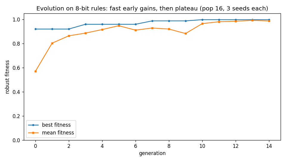
Fitness climbs 0.92 → 1.00 while distinct genomes fall 16 → 3. Improvement and impoverishment arrive together — which is why fitness progress alone never demonstrates discovery, and why the diversity defenses above are load-bearing rather than optional.
Store lineage
Keep parent-child relationships:
record = {
    "generation": generation,
    "genome": genome.tolist(),
    "parent": parent_id,
    "fitness": score,
    "metrics": metrics,
}
Then an evolved rule is not a mysterious final artifact.
We can reconstruct how it emerged.
From evolved rules to learned rules
Evolution changes the rule between simulations.
Later, neural cellular automata will use gradient descent to learn parameters of the local rule.
The optimization mechanism changes, but the surrounding experimental architecture remains recognizable:
parameterized local rule
        ↓
simulation
        ↓
objective
        ↓
update rule parameters
Before we get there, we need one more conceptual piece.
Cellular automata are not only simulations. Some of them can perform computation.
The next chapter looks at information processing, universality and how to think about a cellular automaton as a computer.
Research
Berto, F. & Tagliabue, J. — Cellular Automata (Stanford Encyclopedia of Philosophy). The literature precedent for evolving automata: genetic algorithms searching rule space for computational behavior (Mitchell, Crutchfield & Das), and the Packard/Langton evolution-toward-the-edge-of-chaos program with Mitchell’s critical replication — the tradition this chapter’s loop joins, caveats included. https://plato.stanford.edu/entries/cellular-automata/
Lehman, J. & Stanley, K. O. — Abandoning Objectives (Evolutionary Computation 19(2), 2011). The backing for the diversity section: fixed objectives deceive, and rewarding behavioral novelty finds what pure fitness climbing misses. Pair with the objective-hacking section — they are two halves of one warning. https://dl.acm.org/doi/10.1162/EVCO_a_00025