Neighborhoods as Convolution Kernels
A neighborhood does not have to be a list of nearby coordinates.
It can be a spatial weighting function.
That lets us say:
cells near this radius matter a lot
cells closer in matter less
cells farther away do not matter at all
The standard programming tool for applying that same weighted neighborhood everywhere is convolution.
Start with a small kernel
import numpy as np

kernel = np.array([
    [0.0, 0.1, 0.0],
    [0.1, 0.6, 0.1],
    [0.0, 0.1, 0.0],
])
Normalize it:
kernel = kernel / kernel.sum()
A neighborhood value is now a weighted sum rather than a count. Normalization keeps perception on the state’s own scale: with weights summing to one, a uniform field perceives exactly its own value.
Convolution with periodic boundaries
For teaching purposes, we can write convolution directly:
def periodic_convolve(state, kernel):
    kh, kw = kernel.shape
    cy, cx = kh // 2, kw // 2

    result = np.zeros_like(state, dtype=np.float64)

    for ky in range(kh):
        for kx in range(kw):
            weight = kernel[ky, kx]
            if weight == 0:
                continue

            dy = ky - cy
            dx = kx - cx
            shifted = np.roll(np.roll(state, dy, axis=0), dx, axis=1)
            result += weight * shifted

    return result
This makes the mechanics explicit.
Later we can replace it with FFT convolution for speed without changing the model.
Build a radial kernel
Lenia-style neighborhoods are usually easier to describe in terms of distance from the center.
def radial_coordinates(radius):
    y, x = np.mgrid[-radius:radius+1, -radius:radius+1]
    r = np.sqrt(x*x + y*y) / radius
    return r
Now define a ring-shaped weighting function:
def ring_kernel(radius=15, ring_center=0.5, ring_width=0.15):
    r = radial_coordinates(radius)

    kernel = np.exp(
        -((r - ring_center) ** 2) / (2 * ring_width ** 2)
    )

    kernel[r > 1.0] = 0.0
    kernel[r == 0.0] = 0.0
    kernel /= kernel.sum()

    return kernel
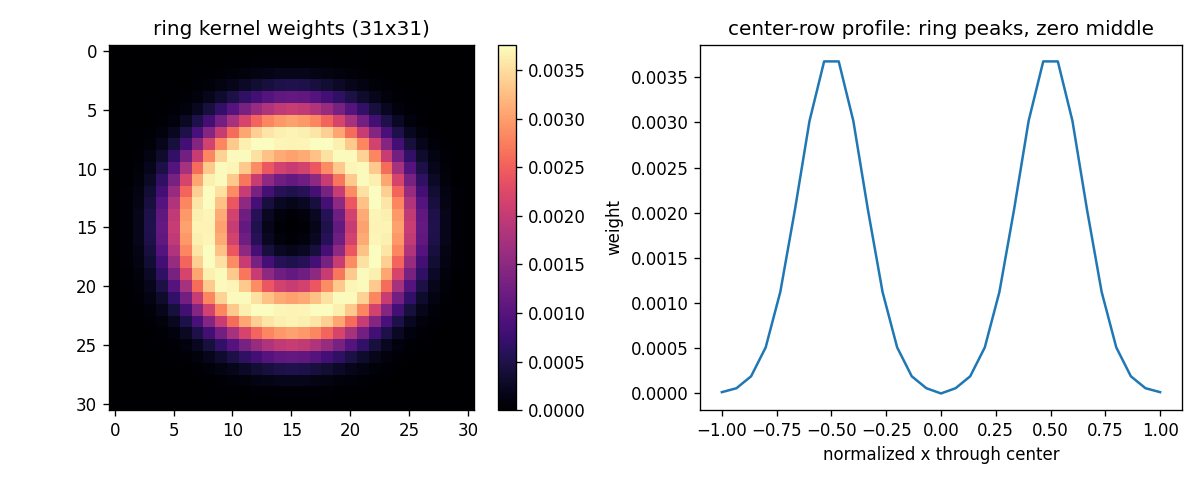
(Verified: sums to exactly 1.0; zero outside the radius; the center cell itself is excluded by this book’s convention — a design choice, stated here so later kernel comparisons use the same baseline.)
Visualize it:
import matplotlib.pyplot as plt

kernel = ring_kernel()
plt.imshow(kernel, cmap="magma")
plt.colorbar()
plt.show()
The neighborhood is now a smooth ring rather than a 3x3 stencil — shown here as a heatmap with its center-row profile, generated from the constructor above:
Every kernel property below is a stated choice with a checkable consequence:
| Property | Value here | Effect | Caveat |
|---|---|---|---|
| normalization | sums to 1.0 | uniform fields perceive themselves | unnormalized kernels rescale all growth |
| center | excluded (0.0) | no self-weight; pure surround | differs from some canonical kernels |
| support | zero beyond radius | finite, compact perception | hard edge at r = 1.0 |
| shape | Gaussian ring at 0.5 | preferred interaction scale | single scale until multi-ring |
Why a ring?
A ring creates a preferred interaction scale.
Instead of asking:
what is immediately adjacent?
we ask:
how much activity exists around this characteristic radius?
That encourages spatial structures with a natural size.
This is one reason continuous artificial-life patterns can look organism-like rather than pixel-like. The word “look” is doing real work in that sentence: a pattern that resembles an organism is not one.
Neighborhood response
Given a state field:
state = np.zeros((128, 128))
state[60:68, 60:68] = 1.0
compute the neighborhood field:
neighborhood = periodic_convolve(state, kernel)
Now every cell has a continuous perception value.
state(x, y)
    ↓
convolution kernel
    ↓
neighborhood potential U(x, y)
This U field is what our growth rule will inspect.
Separate perception from reaction
This architecture is crucial:
state
  ↓
kernel
  ↓
perception field
  ↓
growth function
  ↓
state update
The kernel answers:
What local information reaches this cell?
The growth function answers:
Given that information, should this cell increase or decrease?
Keeping these separate makes the system much easier to reason about and search.
Multiple rings
A kernel can have more than one preferred distance.
def multi_ring_kernel(radius=20):
    r = radial_coordinates(radius)

    inner = np.exp(-((r - 0.35) ** 2) / (2 * 0.08 ** 2))
    outer = 0.6 * np.exp(-((r - 0.72) ** 2) / (2 * 0.10 ** 2))

    kernel = inner + outer
    kernel[r > 1.0] = 0.0
    kernel /= kernel.sum()
    return kernel
Now local interaction has multiple spatial scales.
FFT convolution
The direct implementation costs roughly:
grid cells × kernel cells
That becomes expensive when both are large.
Convolution can also be computed in the frequency domain:
convolution(a, b)
=
IFFT( FFT(a) * FFT(b) )
A compact periodic implementation is:
def fft_convolve(state, kernel):
    padded = np.zeros_like(state)
    kh, kw = kernel.shape
    padded[:kh, :kw] = kernel

    padded = np.roll(padded, -(kh // 2), axis=0)
    padded = np.roll(padded, -(kw // 2), axis=1)

    return np.fft.ifft2(
        np.fft.fft2(state) * np.fft.fft2(padded)
    ).real
Note the parentheses: -(kh // 2), not -kh // 2 — Python floors negative division, so the unparenthesized form misaligns odd-sized kernels by one cell. Centering bugs like this are silent: the output still looks like a blur, just a shifted one.
For production code we would test alignment carefully and probably precompute the kernel FFT.
The important point is architectural:
same model
faster implementation
Test the implementation
Never trust a fast convolution until it agrees with a simple reference implementation.
small_state = np.random.default_rng(1).random((32, 32))
small_kernel = ring_kernel(radius=3)

a = periodic_convolve(small_state, small_kernel)
b = fft_convolve(small_state, small_kernel)

print(np.max(np.abs(a - b)))
(Verified: maximum disagreement ≈ 4e-16 across radii 3, 7, and 15 — machine precision, not visual similarity.)
Performance work should preserve semantics.
The neighborhood is now part of the genome
When we search continuous CA, we are no longer searching only a transition table.
We may search:
kernel radius
ring positions
ring widths
ring weights
growth center
growth width
time step
That is a much richer rule space.
Part III’s search machinery is about to become essential.
We still need a response function
The kernel gives us perception.
But perception alone does nothing.
We need to decide which neighborhood values produce growth and which produce decay.
That mapping is the next major component of Lenia.
In the next chapter we will build growth functions, inspect their geometry, and see how a narrow preference curve can stabilize patterns that would otherwise either disappear or flood the entire world.
Research
Zenil, H. & Martinez, G. J. — Cellular Automata (Scholarpedia). The geometry half of this chapter’s license: automata defined beyond rectangular lattices (triangular, hexagonal, aperiodic, hyperbolic) show neighborhoods are design choices with stated conventions — the tradition this chapter’s kernel-as-function continues, with normalization and centering stated instead of assumed. http://www.scholarpedia.org/article/Cellular_automata
Berto, F. & Tagliabue, J. — Cellular Automata (Stanford Encyclopedia of Philosophy). The computation half: parallel, distributed updating without a central controller is what makes the perception→reaction split meaningful — locality preserved while the neighborhood itself becomes the expressive dimension. https://plato.stanford.edu/entries/cellular-automata/