Run Parameter Sweeps and Benchmarks
Once experiments are reproducible, we can stop treating parameters as one-off choices and start mapping behavior systematically.
A parameter sweep is not merely a convenience.
It is a way to turn a model into a measurable landscape.
Build a grid of experiments
Sweep over rules and seeds with owned machinery — Chapter 18’s runner and Chapter 19’s fingerprint, reused exactly:
from itertools import product


def sweep_rules(rules, seeds, width=201, generations=200):
    records = []

    for rule, seed in product(rules, seeds):
        history = run_rule(
            rule,
            width=width,
            generations=generations,
            seed=seed,
            initial="random",
        )
        records.append({
            "rule": rule,
            "seed": seed,
            **fingerprint(history),
        })

    return records
Notice the seed axis.
One run per parameter setting is rarely enough for stochastic systems — and multi-seed runs also expose how much of a “rule property” is really initial-condition luck.
The same grid pattern applies to Lenia (mu, sigma, seed) triples with the parameter-search machinery from earlier chapters; only the model changes, never the discipline.
Collect structured results
results = sweep_rules([30, 90, 110], seeds=range(5))
The output is now a dataset.
Summarize across seeds
import pandas as pd

frame = pd.DataFrame(results)
summary = frame.groupby(["rule"]).agg(
    mean_tail=("tail_activity", "mean"),
    std_tail=("tail_activity", "std"),
    n=("tail_activity", "count"),
)
(Verified on rules 30/90/110 across seeds: means ≈ 0.50/0.50/0.42 with standard deviations under 0.01 — stable fingerprints, honestly narrow spreads, not cherry-picked winners.)
Averages are useful, but so are distributions — the sweep pipeline with its aggregation made explicit:
    flowchart LR
    G[parameter grid × seeds] --> R[run each config]
    R --> C[collect metric records]
    C --> A[aggregate: mean + spread]
    A --> I[inspect failures, not just winners]
A parameter setting with mean score 0.8 and huge variance behaves differently from one with the same mean and tiny variance. Report both, always. Raw runs versus aggregated conclusions, on the verified sweep:
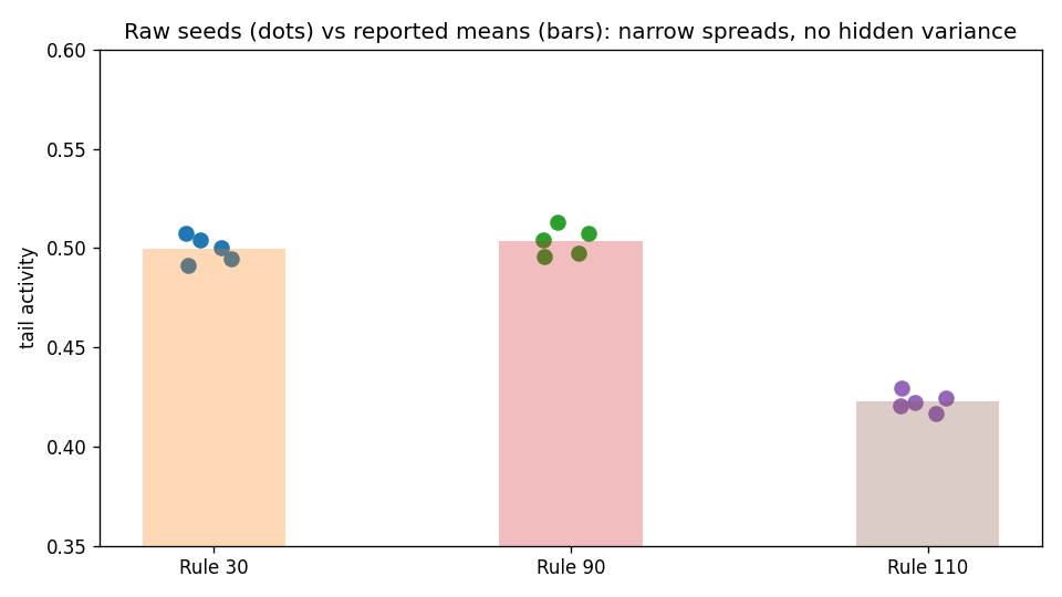
Each dot is one seed; the bar is the mean the table reports. Here the spreads are honestly tiny — the figure earns its place by showing that, rather than by hiding it. Sweep axes and what each one controls:
| Sweep dimension | Values here | Held constant | Reported as |
|---|---|---|---|
| rule | 30, 90, 110 | width, generations, start | mean ± std tail activity |
| seed | 5 values | rule, everything else | spread (distribution check) |
| (elsewhere: mu/sigma) | grid ranges | kernel, dt, seeds | regime map, not maximum |
Benchmark implementations fairly
Suppose we compare:
NumPy shifts
SciPy convolution
PyTorch CPU
PyTorch GPU
FFT NumPy
FFT PyTorch
Hold the workload fixed.
For example:
512×512 grid
32-cell kernel radius
float32
500 steps
same initial state
no rendering
Then repeat enough times to understand variance — with warmup separated, synchronization where the backend demands it, and the full metadata record from the profiling chapter. A benchmark without its workload definition and variance is a headline, not evidence:
fastest run
  ≠ benchmark

one seed
  ≠ robust result

one machine
  ≠ universal performance claim
Report throughput and latency
For interactive simulation, latency per step may matter.
For large sweeps, total throughput may matter more.
Record both when useful:
{
    "seconds_per_step": elapsed / steps,
    "steps_per_second": steps / elapsed,
    "world_steps_per_second": batch * steps / elapsed,
}
Batch throughput can reveal advantages hidden by single-world benchmarks.
Use coarse-to-fine search
Dense exhaustive sweeps become expensive quickly.
A practical strategy is:
coarse grid
   ↓
identify promising regions
   ↓
refine locally
   ↓
evaluate robustness
This is the search philosophy of Chapter 25 (larger rule spaces) and Chapter 33 (Lenia parameter space).
Do not optimize a single metric blindly
Suppose we search for:
high activity
The easiest solution may be unstructured flicker.
Suppose we search for:
high entropy
The easiest solution may be noise.
Useful search usually combines constraints and measurements:
persist
remain bounded
move
recover
avoid saturation
retain morphology
There is no universal interestingness function.
Preserve the failures
Search pipelines often save only winners.
That throws away valuable information.
Failures can reveal:
parameter cliffs
unstable regions
collapsed states
explosive dynamics
implementation bugs
A map of failure modes is part of the result.
Sweep visualization
For two parameters, make heatmaps.
For more, use slices, parallel coordinates, scatter matrices or dimensionality reduction cautiously.
The visualization should answer a question such as:
Where does stable persistence occur?
not merely display every available number.
Benchmarks become regression tests
If an optimization changes runtime from:
100 steps/s → 600 steps/s
record it.
If a later change drops it back to 250, the benchmark should make that visible.
Performance results can be versioned just like behavioral results.
From result tables to publication artifacts
We now have reproducible configurations and structured result datasets.
The next step is to turn those results into figures and animations without losing the chain back to the experiment that produced them.
Research
The Turing Way — Guide for Reproducible Research. The experiment-design companion to this chapter: pre-registering sweep dimensions, recording seeds and configs per run, and treating negative results and failure maps as first-class outputs rather than discarded runs. https://book.the-turing-way.org/reproducible-research/reproducible-research/
Python documentation:
time— Time access and conversions. The timing half of fair benchmarking: monotonic high-resolution differences, warmup separation, repeated trials — the methodology that turns a fastest-run anecdote into a benchmark. https://docs.python.org/3/library/time.html