Vectorize the Update Loop
A cellular automaton is local.
That does not mean we should update it cell by cell in Python.
For dense grids, the same local rule is applied everywhere. That regularity is exactly what array programming is good at.
Start with the obvious implementation
def life_step_slow(grid):
    height, width = grid.shape
    next_grid = np.zeros_like(grid)

    for y in range(height):
        for x in range(width):
            total = 0
            for dy in (-1, 0, 1):
                for dx in (-1, 0, 1):
                    if dx == 0 and dy == 0:
                        continue
                    total += grid[(y + dy) % height, (x + dx) % width]

            alive = grid[y, x] == 1
            next_grid[y, x] = (
                total == 3 or (alive and total == 2)
            )

    return next_grid
This is useful because it states the mechanism clearly.
It is also expensive because Python interprets every nested loop.
Express the neighborhood as array operations
The fast form below is the same rule Chapter 6 already runs — re-derived here as the equivalence target, not a second definition:
def life_neighbors(grid):
    total = np.zeros_like(grid, dtype=np.int16)

    for dy in (-1, 0, 1):
        for dx in (-1, 0, 1):
            if dx == 0 and dy == 0:
                continue
            total += np.roll(np.roll(grid, dy, axis=0), dx, axis=1)

    return total
(np.roll reintroduces wrapped-around elements by definition — which is exactly why every roll-based helper in this book implements periodic boundaries. The boundary semantics come free with the function; changing them requires changing the function.)
The two tiny Python loops now iterate over eight directions, not millions of cells.
Then the rule becomes boolean array logic:
def life_step(grid):
    n = life_neighbors(grid)
    return ((n == 3) | ((grid == 1) & (n == 2))).astype(np.uint8)
Measured on a 48×48 grid: the slow loop takes ≈3ms per step while the vectorized form takes ≈0.09ms — roughly a 33× speedup on one reference machine, for bit-identical output.
Vectorize 1D elementary automata
def elementary_step(state, rule):
    left = np.roll(state, 1)
    right = np.roll(state, -1)

    index = (left << 2) | (state << 1) | right
    bits = np.array([(rule >> i) & 1 for i in range(8)], dtype=np.uint8)

    return bits[index]
No per-cell Python loop is required. (Verified equivalent to the explicit loop for Rule 30 on random states.)
Be aware of temporary arrays
Vectorized code can be faster while allocating more memory.
This expression:
np.roll(np.roll(grid, dy, axis=0), dx, axis=1)
creates temporaries.
For moderate grids that may be fine.
For very large grids or many channels, allocation can become the bottleneck.
Optimization is always workload-dependent.
Use slices when the boundary allows it
If we do not need periodic boundaries, explicit slices can avoid some rolling:
center = grid[1:-1, 1:-1]

neighbors = (
    grid[:-2, :-2] + grid[:-2, 1:-1] + grid[:-2, 2:] +
    grid[1:-1, :-2]                    + grid[1:-1, 2:] +
    grid[2:, :-2]  + grid[2:, 1:-1]  + grid[2:, 2:]
)
The important point is not that slices are universally superior.
It is that boundary semantics and performance strategy interact.
Batch independent worlds
Suppose we want to evaluate 1,000 rules or seeds.
Instead of:
for world in worlds:
    run(world)
we can add a batch axis:
(batch, height, width)
and update many independent worlds in one array operation.
That matters enormously for parameter sweeps and training workloads.
Check equivalence
rng = np.random.default_rng(42)
state = rng.integers(0, 2, size=(64, 64), dtype=np.uint8)

slow = life_step_slow(state)
fast = life_step(state)

assert np.array_equal(slow, fast)
Optimization should be tested against the simplest correct implementation. (Verified: exact equality on random grids.) The optimization workflow as a loop — reference first, speed second, proof always:
    flowchart LR
    R[reference: slow readable loop] --> V[vectorized reformulation]
    V --> E[assert exact equality]
    E -->|pass| B[benchmark both]
    E -->|fail| F[fix, never ship]
    B --> W[keep iff faster at workload sizes]
Measured slow-vs-vectorized scaling (identical outputs, asserted equal every run):
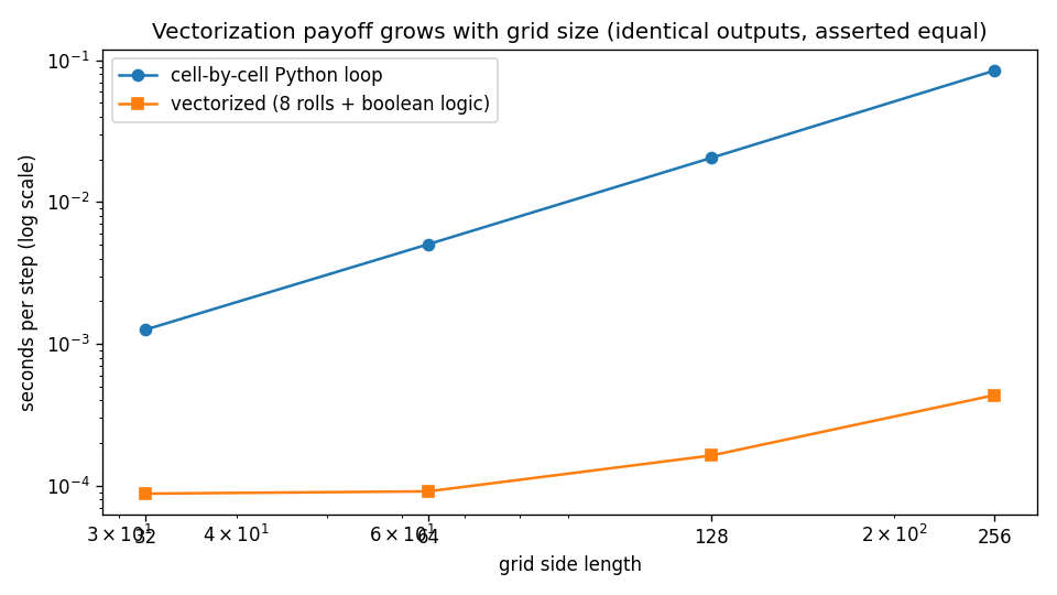
At 256×256 the loop costs ~85ms per step against ~0.4ms vectorized — a ~190× gap that widens with size, because the loop pays per cell while the array form pays per operation.
Implementation options compared — same rule, different cost profiles:
| Implementation | Boundary semantics | Cost shape | Equivalence status |
|---|---|---|---|
| cell-by-cell loop | explicit modulo (any) | per cell, always slow | reference (defines correct) |
| 8 rolls + boolean logic | periodic (roll wraps) | per direction, fast to mid sizes | asserted equal |
| slice arithmetic | fixed/dead edges | no roll temporaries | equal only interior — boundary differs |
| batched (batch, H, W) | inherits inner choice | amortizes per-world overhead | equal per world |
The larger lesson
Cellular automata have an unusually regular computational structure:
same neighborhood operation
same rule
many cells
many steps
That makes them natural candidates for vectorization.
The same structure also makes them natural candidates for GPUs, which is where we go next.
Research
NumPy documentation:
numpy.roll. The exact semantics this chapter’s vectorization stands on: rolled-out elements re-enter at the other side — i.e., every roll-based helper in this book implements periodic boundaries by construction. Check it before assuming any shift-based code shares your boundary model. https://numpy.org/doc/stable/reference/generated/numpy.roll.htmlPython documentation:
time— Time access and conversions. The measurement basis for the speedup claims above:perf_counterdifferences across repeated runs, with warmup separated. Numbers without this discipline are anecdotes. https://docs.python.org/3/library/time.html