Capstone — Discover, Measure and Explain a New System
The previous chapter built the laboratory. This one uses it on a single problem.
The book began with one tiny rule applied to one tiny neighborhood.
We end with a different question:
Can we discover a cellular system, characterize its behavior, test its robustness and explain what we actually know about it?
That is the capstone. It uses the ideas rather than listing them: every stage below reuses owned machinery — Lenia configs and kernels (Ch31), discovery scoring (Ch32), outcome classes (Ch33), the measurement stack (Ch18–22), perturbation discipline (Ch35), search strategy (Ch24–25), and experiment records (Ch55).
Choose a system family
The capstone can use any family we built:
elementary cellular automata
Life-like rules
multi-state rules
stochastic systems
continuous CA
Lenia
neural cellular automata
A strong choice is a parameterized system large enough to contain surprises but small enough to search reproducibly.
For example, single-kernel Lenia over growth parameters with fixed kernel geometry:
search_space = {
    "mu": (0.10, 0.20),
    "sigma": (0.008, 0.04),
    "radius": (8, 24),
    "dt": (0.05, 0.20),
}
State the discovery objective before searching
Do not begin with:
find something cool
Define observable criteria.
For example:
survives 2,000 steps
remains spatially bounded
maintains nonzero activity
moves at least 10 cells
recovers at least 70% after a fixed perturbation
persists on most nearby seeds and small parameter shifts
These criteria do not define life or intelligence.
They define the experiment.
The last criterion belongs on the list before any result exists. A candidate that meets the first five and fails it is a lucky seed, not a discovery. When the champion is rejected later in this chapter, that rejection is this criterion being applied, not a verdict invented after the fact.
Run a reproducible coarse search
Assemble owned pieces — config sampling (Ch33), seed runner (Ch32), scoring and outcome classes (Ch32–33), full experiment records (Ch55):
def sample_candidates(search_space, seed=1234):
    rng = np.random.default_rng(seed)
    # yields LeniaConfig + seed pairs on a coarse grid
    ...


def evaluate_candidate(candidate):
    config, seed_value = candidate
    initial = random_seed(seed=seed_value)
    result = evaluate_seed(initial, config, steps=500)
    return {
        "score": candidate_score(result),
        "outcome": classify_outcome(result),
        "result": result,
    }


for candidate in sample_candidates(search_space, seed=1234):
    result = evaluate_candidate(candidate)
    save_result(candidate, result)
Record every candidate with:
parameters
seed
code version
metrics
termination reason
Then rank without deleting the failures.
Executed on a 3×3 (mu, sigma) grid × 2 seeds: scores spread 0.40–0.66 with outcomes split between persistent-dynamic and dead — the search discriminates rather than flatters, in about a second of compute. The top scorer (mu=0.15, sigma=0.02, score 0.655) becomes the refinement input, not the conclusion.
Refine promising regions
Suppose several candidates cluster near the top scorer, here:
mu ≈ 0.15
sigma ≈ 0.02
Search locally around that region.
coarse discovery
      ↓
local refinement
      ↓
robustness testing
Do not mistake one lucky seed for a stable region of behavior. The neighborhood test below applies the last criterion in the objective, and the coarse winner above dies on two of three nearby seeds. The order is always champion first, region second.
Build a behavioral fingerprint
For each finalist, measure multiple dimensions with the owned stack — mass and activity (Ch28/Ch18), entropy (Ch20), centroid motion (Ch31), compactness from the active mask, damage recovery (Ch35), sensitivity (Ch22):
capstone_fingerprint = {
    "mean_mass": ...,
    "activity": ...,
    "entropy": ...,
    "centroid_speed": ...,
    "compactness": ...,
    "damage_recovery": ...,
    "sensitivity": ...,
}
The point is not to collapse these into one magical complexity score.
The point is to describe the system from several defensible angles.
Test neighboring parameters
If a pattern exists only at one exact floating-point coordinate, that tells us something important.
Evaluate nearby values:
mu ± ε
sigma ± ε
radius ± 1
dt ± ε
Then ask:
Is behavior stable in a region?
Does it change smoothly?
Is there a sharp transition?
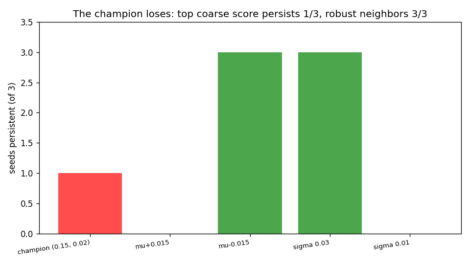
A parameter map is often more informative than the champion itself. Verified on the coarse winner: shifting mu by +0.015 kills all three seeds, narrowing sigma to 0.01 kills all three, while mu −0.015 and sigma +0.01 stay robust — a fragile champion beside genuinely stable neighbors. In this three-seed, 150-step neighborhood test, the coarse winner failed the robustness criterion stated at the outset, and the robust neighbors, not the champion, are what the search found. Three seeds are enough to reject this candidate under the stated test; they are not enough to estimate a general robustness rate.
Perturb the system
Use a perturbation suite rather than one hand-picked success case.
small circular deletion
large deletion
additive noise
translated initial state
changed update rate
larger canvas
Record:
recovery success
recovery time
final morphology error
mass change
continued motion
Now robustness becomes measured behavior — with Chapter 35’s split intact: mass recovery is not morphology recovery, and neither is called regeneration without the training setup that word requires.
Compare against baselines
A discovery is easier to interpret when compared with alternatives.
For example:
candidate
nearby parameter candidate
random parameter candidate
static/persistent baseline
high-activity noise-like baseline
If every random system scores similarly, our metric is not discriminating enough. And the full-flip lesson from Chapter 24 applies verbatim: a degenerate world flipping every cell scores maximal activity at zero entropy — baselines exist to catch exactly this.
Show the failures
The workflow must reject bad results on the record, not just celebrate good ones. From this book’s own verified experiments:
fragile champion (mu=0.15, sigma=0.02):
  top coarse score, dead on most neighboring seeds
  → rejected in favor of a robust region

full-flip degenerate:
  activity 1.0, entropy 0.0
  → maximal score, trivial dynamics; rejected by region constraints

narrow-sigma collapse (sigma=0.01):
  uniform death across seeds
  → extinction zone mapped, not merely a bad run
A map of failure modes is part of the result.
Inspect mechanism where possible
For a hand-designed continuous CA, inspect:
kernel response
growth response
local field distributions
regions of positive/negative update
For an NCA, inspect:
hidden-channel trajectories
probe predictions
channel ablations
spatial shuffles
local interventions
The question is not:
Can we tell a beautiful story about the mechanism?
It is:
Which claims survive intervention and measurement?
Produce the artifact set
A finished capstone should generate at least:
config.json
metrics.csv
behavioral-fingerprint.json
parameter-map.png
representative-state.png
activity-timeseries.png
perturbation-comparison.png
animation.mp4 or gif
README/report.md
Every figure should be traceable to a run.
Write the conclusion in layers
Separate observation from interpretation.
The example below shows the shape of the sentences. Its numbers are placeholders, not results from this book’s experiments:
Observation
The candidate remains bounded for 2,000 steps and its centroid moves 18.4 cells.
Observation
Across 20 circular damage trials, 16 return below the predefined morphology-error threshold.
Interpretation
This behavior is consistent with a persistent mobile structure with measurable regenerative capacity under the tested perturbations.
Then state the limit:
This does not establish biological life, agency or intelligence.
Precision makes the result stronger, not weaker.
What we can claim
The book’s final ledger, in the buckets it earned:
DEMONSTRATED IN THIS BOOK
  some one-byte rules grow irregular histories (Rule 30);
  local rules plus measurement plus search find persistent
  localized patterns in single-ring Lenia, and map where
  they survive;
  every optimization preserved checked semantics or said so.

SUPPORTED BY LITERATURE
  Rule 110's universality under arranged configurations
  (Cook), and the limits of that result;
  Lenia species catalogs and parameter maps;
  NCA growth/persistence/regeneration regimes;
  novelty search outperforming fixed objectives.

OBSERVED IN OUR EXPERIMENTS
  regime maps with robust interiors and fragile borders;
  mass recovery without morphology recovery;
  metric gaming by degenerate worlds;
  seed- and configuration-dependent outcomes throughout.

INTERPRETATION
  emergence as observed behavior from local interaction;
  computational irreducibility as a position, not a theorem;
  edge-of-chaos as a heuristic, not a law.

OPEN QUESTION
  everything the prize problems, the species catalogs,
  and the generalization matrices have not settled —
  which is most of what matters.
The verdicts that matter most, with their evidence status — including the rejection this capstone exists to demonstrate:
| Claim | Evidence | Status |
|---|---|---|
| coarse champion (mu=0.15, σ=0.02) is the best system | top grid score 0.655 | rejected: persistent on 1 of 3 nearby seeds |
| neighboring region (mu=0.135 / σ=0.03) persists | 3 of 3 seeds each | accepted as robust (within tested neighborhood) |
| narrow sigma (0.01) is viable | 0 of 3 seeds survive | rejected: extinction zone mapped |
| mass recovery implies repair | mass 0.76→1.00, IoU fluctuating | rejected: morphology did not follow |
| full-flip worlds are interesting | activity 1.0, entropy 0.0 | rejected: degenerate by region constraints |
The rejection, plotted — persistence across the champion’s neighborhood (3 seeds each, 150 steps):
The method that produced every verdict above, stated once as the book’s closing loop:
    flowchart LR
    C[construct candidate] --> O[observe behavior]
    O --> M[measure: fingerprint + metrics]
    M --> H[challenge: neighbors, damage, baselines]
    H --> V{evidence holds?}
    V -->|yes| A[accept provisionally]
    V -->|no| R[reject + record why]
    R --> C
The entire book in one workflow
We can now summarize the journey:
local state
    ↓
local neighborhood
    ↓
local rule
    ↓
repeated dynamics
    ↓
emergence
    ↓
measurement
    ↓
search
    ↓
artificial life
    ↓
learned local rules
    ↓
robustness and generalization
    ↓
reproducible experimentation
    ↓
challenge, verification, rejection
The deepest idea has remained unchanged from the first chapter:
Complex global behavior can arise from simple local interactions.
But we have added a second principle that matters just as much:
Interesting behavior becomes knowledge only when we can reproduce, measure, challenge and explain it.
That is where cellular automata stop being merely fascinating pictures and become a laboratory for computation, emergence and self-organization — with the laboratory, not the pictures, as the endpoint.
Research
Wolfram, S. — Statistical Mechanics of Cellular Automata (Reviews of Modern Physics 55, 1983). Foundations: the first exhaustive rule-space survey — the methodological ancestor of every scan, sweep, and catalog in this book. https://doi.org/10.1103/RevModPhys.55.601
Berto, F. & Tagliabue, J. — Cellular Automata (Stanford Encyclopedia of Philosophy). Conceptual frame: definitions, computation, emergence, and the philosophical uses and abuses the capstone’s layered conclusion is built to avoid. https://plato.stanford.edu/entries/cellular-automata/
Cook, M. — Universality in Elementary Cellular Automata (Complex Systems 15(1), 2004). Universality anchor: what “can compute” means at its strongest, and under which arranged conditions. https://doi.org/10.25088/ComplexSystems.15.1.1
Chan, B. W.-C. — Lenia: Biology of Artificial Life (Complex Systems 28(3), 2019). Continuous ALife: the system family the capstone searches, with species, maps, and caveated biological vocabulary. https://arxiv.org/html/1812.05433v3
Mordvintsev, A., Randazzo, E., Niklasson, E. & Levin, M. — Growing Neural Cellular Automata (Distill, 2020). Learned CA: growth, persistence, and regeneration as trainable regimes — the strongest version of “design the objective, learn the rule.” https://doi.org/10.23915/distill.00023
Earle, S., Yildiz, O., Togelius, J. & Hegde, C. — Pathfinding Neural Cellular Automata (2023). Algorithmic generalization: learned local procedures tested where training ends — the standard for any capstone claim about computation beyond examples. https://arxiv.org/abs/2301.06820
Lehman, J. & Stanley, K. O. — Abandoning Objectives (Evolutionary Computation 19(2), 2011). Search philosophy: novelty over fixed scores — the reason the capstone maps regions instead of crowning champions. https://dl.acm.org/doi/10.1162/EVCO_a_00025
The Turing Way — Guide for Reproducible Research. Experiment discipline: configurations, run identity, raw-before-derived artifacts — without which the capstone is a demo, not a result. https://book.the-turing-way.org/reproducible-research/reproducible-research/