Classify Rule Behavior
We now have six kinds of measurement. The literature already offers a coarser tool for organizing rules: four broad behavioral classes.
Class I   -> settles to homogeneous behavior
Class II  -> settles to simple stable or periodic structures
Class III -> irregular, apparently random behavior
Class IV  -> persistent local structures and complex interactions
These labels are useful vocabulary — phenomenological shorthand from Wolfram’s 1980s survey, not formal dynamical-systems theorems. “Class III” here means Wolfram-class irregularity, not proven chaos in the mathematical sense; the book has called Rule 30 “irregular” until now for exactly this reason, and this chapter does not upgrade that word.
Each label, what it describes, and what it never establishes:
| Class | Phenomenology | Often read as | Does not prove |
|---|---|---|---|
| I | settles homogeneous | “simple” | uninteresting in all setups |
| II | stable or periodic structures | “ordered” | absence of computation |
| III | irregular, apparently random | “chaotic” | formal chaos, randomness theorem |
| IV | localized persistent structures | “complex, universal” | universality, optimality |
But if we want to use them experimentally, we should connect them to measurable evidence rather than treating them as magic categories.
Start with features
For each rule, assemble one record from the owned observables — fingerprint (Chapter 19) for density/activity/persistence, entropy (Chapter 20), compression (Chapter 20), recurrence (Chapter 21):
def rule_features(history):
    features = fingerprint(history)

    features["mean_entropy"] = float(
        entropy_curve(history).mean()
    )
    features["compression_ratio"] = compression_ratio(
        history
    )
    features.update(recurrence_metrics(history))

    return features
Each feature captures a different aspect of the dynamics, and every key traces to exactly one owner chapter. Sensitivity from Chapter 22 joins selectively: it costs fifty paired runs per rule, so it belongs on shortlists, not on all 256. Where it is wanted, add it to the record explicitly:
features = rule_features(history)
features["sensitivity"] = sensitivity_trials(rule_number)
Heuristics before machine learning
A first classifier can be explicit and inspectable:
def rough_class(metrics):
    if metrics["tail_activity"] < 0.01:
        if metrics["mean_entropy"] < 0.1:
            return "I"
        return "II"

    if metrics["sensitivity"] > 0.35 and metrics["compression_ratio"] > 0.6:
        return "III"

    return "IV-candidate"
The compression threshold is calibrated to this book’s own packbits+zlib representation — measured ratios run from ≈0.01 (frozen rules) through Rule 30 at ≈0.73 to ≈1.0 (pure noise), so 0.6 separates sustained irregularity from the middle. A different representation would need a different number.
This is deliberately approximate.
The point is not that these thresholds define the canonical classes.
The point is to make our assumptions visible. (Checked: with measured values, Rule 30 lands III and Rule 110 lands IV-candidate — sane, while borderline cases like single-car Rule 184 expose the roughness honestly.)
As a decision flow — thresholds first, humility built in:
    flowchart TD
    F[feature record] --> T{tail activity < 0.01?}
    T -->|yes| E{mean entropy < 0.1?}
    T -->|no| S{sensitivity > 0.35 and compression > 0.6?}
    E -->|yes| C1[class I]
    E -->|no| C2[class II]
    S -->|yes| C3[class III]
    S -->|no| C4[IV-candidate: needs structural evidence]
Why Class IV is hard
Class IV behavior is often described in terms of localized structures, interactions and long transients.
Those are harder to capture with simple global statistics.
A rule can have moderate entropy and activity without containing coherent objects. So a useful Class IV detector may need richer features:
localized persistence
moving motifs
collision diversity
long transient lengths
spatial mutual information
compressible background + irregular structures
This is a research problem, not a one-line threshold. Note the guardrails such a detector must respect:
Class IV
  ≠ computational universality

Class IV
  ≠ optimal complexity

visual appearance
  ≠ unique dynamical class
Rule 110 is both Class IV and universal, but the first fact did not prove the second — Cook’s construction did. Conflating them turns a visual label into a theorem.
Plot feature space
Even two features can reveal clusters — measured here for all 256 rules from single-cell starts (101 cells, 120 generations):
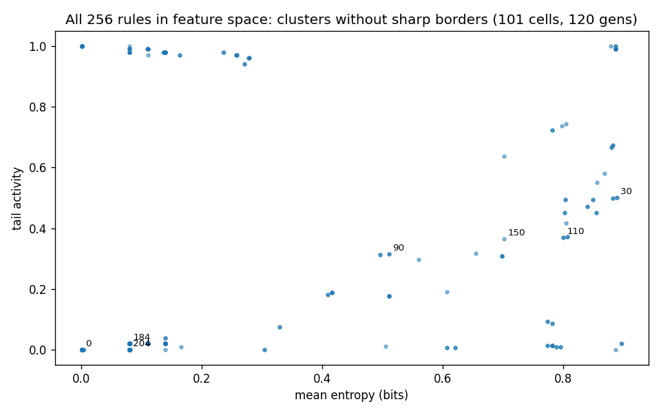
Rules that looked unrelated by rule number sit close together behaviorally — and the famous rules (0, 30, 90, 110, 150, 184, 204) scatter across the cloud rather than occupying neat territories. Any threshold line drawn through this space, including this chapter’s own, is a heuristic cut through continuous variation — which is exactly why the classifier reports candidates, not verdicts.
import matplotlib.pyplot as plt

x = [row["mean_entropy"] for row in records]
y = [row["tail_activity"] for row in records]
labels = [row["rule"] for row in records]

plt.scatter(x, y)
plt.xlabel("mean entropy")
plt.ylabel("tail activity")
plt.show()
Add sensitivity or compression as a third dimension in separate plots.
Standardize before comparing distances
Metrics have different ranges.
If we calculate Euclidean distance directly, one large-scale feature can dominate.
Standardize them:
X = np.array([
    [
        row["mean_density"],
        row["mean_change"],
        row["mean_entropy"],
        row["compression_ratio"],
        row["sensitivity"],
    ]
    for row in records
])

X = (X - X.mean(axis=0)) / (X.std(axis=0) + 1e-9)
Now nearest-neighbor comparisons become more meaningful.
Classification versus discovery
Classification asks:
Which known category does this rule resemble?
Discovery asks:
Which rules behave unusually relative to the rest?
The second question may be more interesting.
Compute distance from the feature-space mean or from nearby clusters and inspect outliers.
An unexpected rule is often more valuable than a rule that cleanly fits a label.
Keep the evidence
If a program labels Rule 110 as a Class IV candidate, store the measurements that caused the decision.
classification = {
    "rule": 110,
    "label": "IV-candidate",
    "evidence": metrics,
    "classifier": "rough-v1",
}
This makes the classification reproducible and revisable.
Next: exhaustive search
For elementary cellular automata, the entire rule space contains only 256 rules.
That is tiny enough to evaluate exhaustively.
In the next chapter we will stop choosing famous rules by name and let Python run every rule, measure every run, rank candidates and generate an experimental catalog.
Research
Zenil, H. & Martinez, G. J. — Cellular Automata (Scholarpedia). The literature behind this chapter’s caution: Wolfram’s four classes are heuristic descriptions dependent on initial conditions, observation time, and measurement — with quantitative follow-ups (statistical, basin, compression-based) and explicit limitations. The reference for keeping “Class III” and formal chaos apart. http://www.scholarpedia.org/article/Cellular_automata
Berto, F. & Tagliabue, J. — Cellular Automata (Stanford Encyclopedia of Philosophy). Places the classes in history (Wolfram’s 1980s taxonomy of the 256 rules) and qualifies them the way this chapter does: Class IV’s association with universal computation is a conjecture-backed observation about specific rules, proved case by case — never a property of the label. https://plato.stanford.edu/entries/cellular-automata/